Regional Employment Structure Using Labor Market Centrality Index
This post is based on joint work with Dr. Kate Nesse, and is published in the Internation Regional Science Review.
Introduction
Office of Managment and Budget (OMB) identifies Core Based Statistical Areas (CBSA) as collections of counties. These CBSA can be Metropolitan (MSA) or Micropolitan \(\mu\)SA based on the population of the ‘core’ (\(\ge\) 50,000 or not). Within these Statistical Areas, counties can either be Central (contain all or a substantial portion of the urbanised area) or Outlying (employment interchange measure with the Central counties above 25%). In other words, the centrality of the county is defined by the urban population attributes of the county rather than its relative location in the commuting network, whereas Outlying defined in relation to the Central counties. In 2015, a vast majority of the counties within CBSA are considered Central; only 29% of the counties are Peripheral/Outlying. This is even more stark within \(\mu\)SAs where only 14% are considered Peripheral. CBSAs are predominantly dominated by the Central counties; they account for 92.5% of the CBSA population. These Central counties are crucial to the delineation of these statistical regions and encompass the economic core of the country.
Table 1 Types of CBSAs and Counties in Conterminous United States. Source: OMB (2015)
| County Type | |||
|---|---|---|---|
| CBSA Type | Central | Outlying | Total |
| MSA | 785 | 451 | 1,236 |
| \(\mu\)SA | 569 | 94 | 663 |
| Total | 1,354 | 545 | 1,899 |
These definitions are built upon the assumption that a labor market is built around a central node. While this may have been the case historically, with our increasingly complex cities and multiplicity of transportation networks, contemporary cities have much more complex labor market networks and regional structures. In this work, we examine if a different approach to defining the core would affect our understanding of the economic geography of metropolitan United States. In particular, we are interested in understanding how the positionality of the nodes in the network illuminates our understanding of the regions.
Labor Market Centrality Index
A k–core of an unweighted simple binary graph is its subgraph where all the nodes have at least degree \(k\). This subgraph is obtained by iteratively removing nodes from the network whose degree is less than k until a stable set of vertices with the minimum degree is reached. A node in a network has a coreness index \(k\), if it belongs to a \(k\)–core but not a \(k+1\)–core.
This can be generalized to a directed network by focusing on the indegree; i.e. a \(k\)–core is the subgraph, where all nodes have an in-degree \(k\). We can also generalize this concept to a weighted graph by using \(s\)–core decomposition, where degree of the vertex is replaced by strength of the vertices (Eidsaa and Almaas 2013). If, the edge weight between nodes \(i\) and \(j\) is denoted by a non-negative \(w_{ij}\), then the strength of the vertex \(i\)$is defined as
\[ s_i = \sum_{j \in N_i^-} w_{ij} \]
where \(N_i^-\) is the in-neighborhood of \(i\) . The \(s\)-core is a subgraph where the nodes have at least strength \(s\). As long as \(w_{ij} \in Z^+\), we can replace an edge in the graph with \(w_{ij}\) multi-edges, and the decomposition of the graph by strength and degree are equivalent. We call this coreness index, the labor market centrality index when applied to commuting networks.

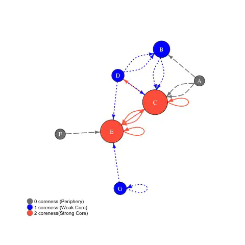
Illustration of network decomposition into core and periphery. Vertices are sized based on in-degree.
The s–core decomposition is illustrated in the above figure for directed graph with multiple edges including loops. The entire graph in the figure is part of 0-core. Nodes A and F have in-degree 0, and therefore are not part of the 1-core of the graph (subgraph induced by nodes B, C, D, E, G). Thus, the coreness of A and F is 0. In that 1-core of the subgraph, nodes D and G have in-degree 1. While they are not part of the 2-core of the graph, deleting them also renders B ineligible for 2-core. Thus, the coreness index of nodes B, D and G is 1. This process continues, till all nodes are assigned a coreness index. The vertices in the top 10 percentile of the index is classified as strong core and in the upper quartile, but not in the upper decile as weak core. The rest are periphery.
We use the 2011–2015 county-to-county commuting flow data from the American Community Survey. For the sake of exposition, we limit our analysis to the conterminous United States consisting of 3,109 counties. 134,869 pairs of counties have non-zero commuters, representing 1.4% of the possible links; the network is relatively sparse, a testament to the continuing importance of geographic distance for economic integration. These links represent 142.5 million commuters, of which 72% commuted within the same county. When the above coreness index is computed on this dataset, we call it Labor Market Centrality Index.
Core & Periphery Structure of the United States
The Labor Market Centrality Index based on 2015 ACS commuting data (logrithmically transformed) is above for the conterminous United States. The results point to tightly connected large cores in the Northeastern United States that span Boston to Washington, D.C.; in Florida around Miami and Tampa; in Southern California around Los Angeles; and in Northern California around San Francisco (see Figure 2). As can be expected, there are also numerous other smaller cores around Miami, Atlanta, Chicago, Detroit, Seattle, Denver and other cities.
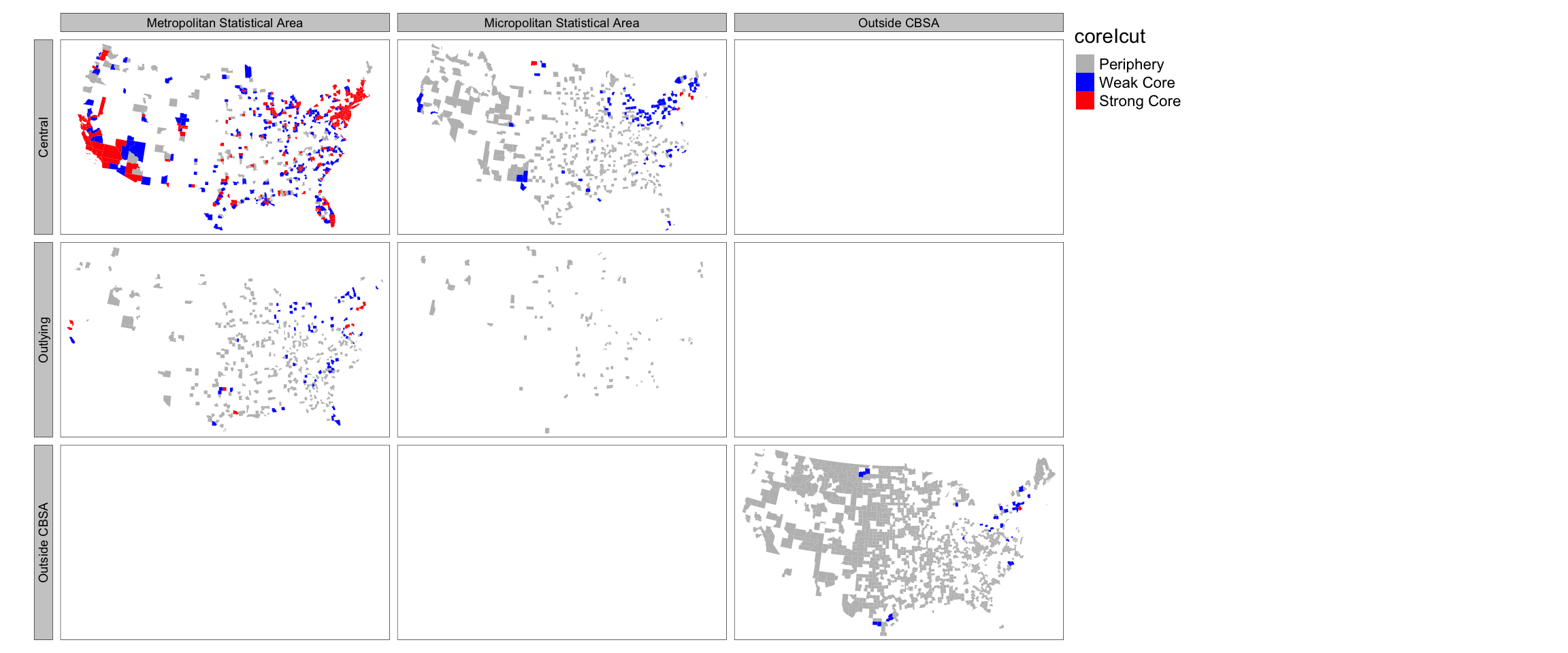
280 counties are classified as Strong Core and 471 are classified as Weak Core. The rest are in the peripheral (see above maps). There are 92 distinct geographical clusters of Strong Core counties (defined by queen contiguity), with the biggest one comprising of 109 counties stretching from Portland, Maine to Northern Virginia. The second biggest cluster is the 28-county collection in California, from San Diego to Santa Rosa. The rest of the geographic clusters are comprised of 1 to 7 counties, with 65% of them being a single county. With the inclusion of weak core counties, the number of geographic clusters to increases to 108: 23 of the clusters are a collection of weak and strong core counties; 49 of the clusters are only comprised of weak core counties.
There is one county (Sullivan, New York) that is not part any CBSA but belongs to a strong core. 11 outlying counties, as defined by OMB, belong to strong core. Similarly, two counties in New York, and one each in Connecticut, Pennsylvania and North Dakota are part of \(\mu\)SAs, but are part of strong core. More importantly, 638 central counties (OMB characterization) are not part of strong or weak core (see above maps). While these counties have urban populations above the thresholds specified, they have fewer commuters both to other nodes as well as to themselves, implying a comparatively weak local and regional economy. These disagreements in classifications provide a productive starting point to analyze the role of ‘small’ non-urban counties in the regional economy as well as large urban counties that are experiencing economic stagnation and decline.
Why Bother?
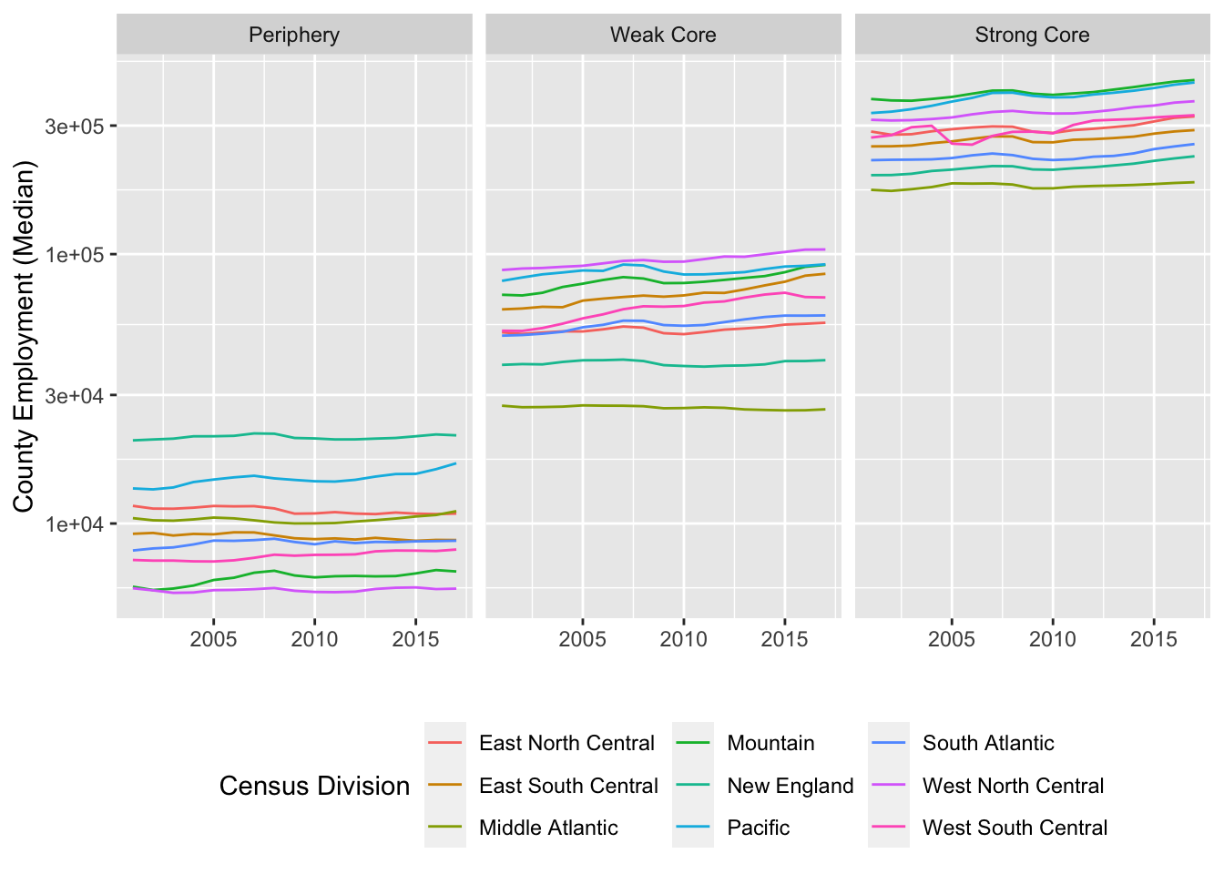
To see why this classification may be more useful, it is illustrative to see changes in the employment pre and post-recession in different types of counties (See figure below). While the Weak Core counties grew (in terms of number of jobs) roughly at the same rate as the Strong Core counties pre-recession (2001-2008), the recovery in the post-recession has been twice as strong in the Strong Core counties in the post-recession. The recovery seems to have bypassed the Periphery counties; while they grew at a healthy 3% before the recession, they contracted by 0.5% after the recession. In part, these numbers can be explained due the spatial sorting of specializations and the changing nature of the economy. However, these distinctions are not as stark, if we use the Central and Outlying distinctions of OMB. Central counties (on average) marginally grew faster compared to Outlying counties (1.6% vs. 0.63%) during the post-recession, even while they had similar growth rates pre-recession (6.75 vs. 6.45). However, Central counties with MSA significantly outpaced Central counties within µSA in post-recession recovery (4.3% vs. -0.84%). This, together with the specialization in service industries indicates that it is not the population size of the county that is related to the economy but rather its place in the regional network. We do not make any claims as to the causal relationship between the position in the network and the economic growth.
Conclusions
There are many ways to understand human settlements. In this paper, we looked at the regional structure from a network perspective. We found that how a county functions within the network of human settlement across the continental US is based on population and economic activity. Our typology reflects economic dimensions in addition to population and density.
Metropolitan regions are formed around economic activity and therefore reflect economic centers but existing typologies do not characterize the strength and nature of the regional economy well. Focusing on the role of the county in the network through commute patterns illuminates not just how central a county is in the labor market but also broadly demonstrates the strength of the economy. This is independent of the size of the population. Although there is some relationship between the size of the population and the size of the economy, there were some small counties with a lot of commute flows and large counties that had very little commuting. Categorizing counties based on their function in the network of human settlements is a useful way to understand the integration of population and economy. It shares some similarities with other typologies focused on commuting flows. However, it has the unique feature of reflecting the economic strength of the region in a more dynamic way than other categorization and indices.
Nikhil Kaza
Professor
My research interests include urbanization patterns, local energy policy and equity