Finding Pedestrians with Tiled Windows
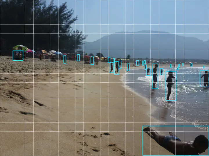
Introduction
In the previous post, we ran a pre-trained YOLO26 model on street-level photographs from Rio de Janeiro, entirely in R. The model accepts exactly one input size, 640 × 640 pixels, so every photograph was shrunk to fit. A 3,232 × 2,424 photograph was reduced by a factor of five in each direction, which means every 25 pixels of the original became one pixel for the model.
For a car in the foreground, that doesn’t matter. For a pedestrian half a block away, it can mean the difference between being counted and being missed. A person who is 100 pixels tall in the photograph is 20 pixels tall by the time the model sees them. Pedestrians are exactly the road users that planners most often want to count and that cameras mounted on cars are most likely to miss.
This post takes a different approach. Instead of shrinking the whole photograph, we cut it into overlapping tiled windows and look at each one in turn. Each window is 640 × 640 pixels of the original photograph, so the model sees every part of it at full resolution. We then combine the detections from all the windows into a single set, throwing out the duplicates. In the computer vision literature this is known as sliced inference; one widely used implementation is SAHI.
Setup
This post uses the same packages, model and class table as the previous one.
library(torch)
library(terra)
library(tidyverse)
library(here)
If you are following along, download the exported model, yolo26s.torchscript and the COCO class table, coco_classes.csv, and save both in your InputData folder.
model        <- here("InputData", "yolo26s.torchscript") %>% jit_load()
coco_classes <- here("InputData", "coco_classes.csv") %>% read_csv(show_col_types = FALSE)
IMG_SIZE    <- 640L   # the model's fixed input size
PAD_VALUE   <- 114    # grey padding
CONF_THRESH <- 0.5
The functions below are the ones we built in the previous post, with one change. They take a raster rather than a file path, because a window is a piece of a raster, not a file. detect_raster() returns only pedestrians (the person class), in the pixel coordinates of whatever raster it was given, with y counting down from the top.
read_photo <- function(path) {
    r <- rast(path)
    ext(r) <- ext(0, ncol(r), 0, nrow(r))   # pixel units; GDAL needs an explicit extent
    names(r) <- c("red", "green", "blue")
    r
}

letterbox <- function(r, size = IMG_SIZE) {
    w <- ncol(r); h <- nrow(r)
    ext(r) <- ext(0, w, 0, h)   # local pixel coordinates, even for a window

    scale <- min(size / w, size / h)
    new_w <- round(w * scale); new_h <- round(h * scale)
    template <- rast(nrows = new_h, ncols = new_w, nlyrs = 3, extent = ext(r), crs = crs(r))
    resized <- resample(r, template, method = "average")

    left <- (size - new_w) %/% 2L; top <- (size - new_h) %/% 2L
    ext(resized) <- ext(left, left + new_w, size - top - new_h, size - top)
    padded <- extend(resized, ext(0, size, 0, size), fill = PAD_VALUE)

    list(raster = padded, scale = scale, left = left, top = top)
}

raster_to_tensor <- function(r) {
    torch_tensor(aperm(as.array(r), c(3, 1, 2)), dtype = torch_float32())$div(255)$unsqueeze(1)
}

detect_raster <- function(r, conf_thresh = CONF_THRESH, classes = "person") {
    lb <- letterbox(r)
    pred <- as.matrix(with_no_grad(model(raster_to_tensor(lb$raster)))$squeeze(1))

    keep  <- pred[, 5] > conf_thresh
    boxes <- pred[keep, 1:4, drop = FALSE]
    boxes[, c(1, 3)] <- (boxes[, c(1, 3)] - lb$left) / lb$scale
    boxes[, c(2, 4)] <- (boxes[, c(2, 4)] - lb$top)  / lb$scale

    tibble(
        xmin = boxes[, 1], ymin = boxes[, 2],
        xmax = boxes[, 3], ymax = boxes[, 4],
        conf = pred[keep, 5],
        class_id = pred[keep, 6]
    ) %>%
        left_join(coco_classes, by = "class_id", relationship = "many-to-one") %>%
        filter(class %in% classes)
}

plot_detections <- function(r, dets, main = NULL, col = "cyan") {
    ext(r) <- ext(0, ncol(r), 0, nrow(r))
    h <- nrow(r)
    plotRGB(r, mar = c(0, 0, if (is.null(main)) 0 else 1.5, 0))
    if (!is.null(main)) title(main, line = 0.2, cex.main = 1)
    if (nrow(dets) == 0) return(invisible())
    rect(dets$xmin, h - dets$ymax, dets$xmax, h - dets$ymin, border = col, lwd = 1.5)
}
Two photographs
We use the same street-level images from Rio de Janeiro as the previous post, unzipped into your InputData folder.
img_files_paths <- here("InputData", "geotagged") %>%
    list.files(full.names = TRUE, pattern = "\\.jpg$")
street_path <- img_files_paths[str_detect(img_files_paths, "1318415481")]
beach_path  <- img_files_paths[str_detect(img_files_paths, "1319660481")]

street <- read_photo(street_path)
beach  <- read_photo(beach_path)
dim(street)
# [1] 2424 3232    3
dim(beach)
# [1] 2988 3984    3
The first photograph was taken through the windscreen of a bus on a busy commercial street. The second is a beach, with people scattered along the shoreline at different distances from the camera. Here is what a single pass of the model finds in each.
street_single <- detect_raster(street)
beach_single  <- detect_raster(beach)

par(mfrow = c(1, 2))
plot_detections(street, street_single, paste("street, single pass:", nrow(street_single)))
plot_detections(beach,  beach_single,  paste("beach, single pass:", nrow(beach_single)))
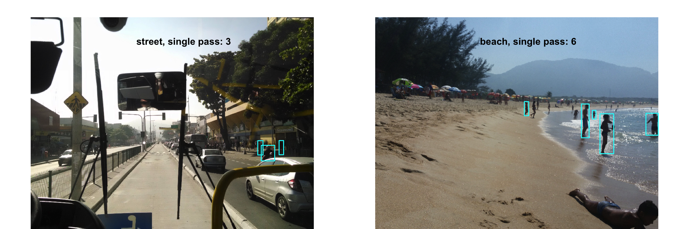
In both photographs you can see many more people than the model found.
What the single pass loses
Let’s look closely at the pavement on the right of the street photograph, where the model found a few people. We crop a region around those detections, and compare it at full resolution with the same region at the resolution the model actually saw.
h <- nrow(street)
zoom <- ext(min(street_single$xmin) - 400, max(street_single$xmax) + 300,
            h - max(street_single$ymax) - 150, h - min(street_single$ymin) + 150)
zoom <- terra::intersect(zoom, ext(street))   # keep the region inside the photograph

scale <- IMG_SIZE / max(dim(street)[1:2])
template <- rast(nrows = round(nrow(street) * scale), ncols = round(ncol(street) * scale),
                 nlyrs = 3, extent = ext(street), crs = crs(street))
street_seen <- resample(street, template, method = "average")   # what the model saw

full_crop <- crop(street, zoom)
seen_crop <- crop(street_seen, zoom)
dim(full_crop)
# [1] 532 994   3
dim(seen_crop)
# [1] 105 197   3
Because street_seen covers the same extent as street, only with larger cells, the same extent zoom crops the same part of the scene from both. The two crops cover identical ground, but one has 528,808 pixels in each band and the other 20,685.
par(mfrow = c(1, 2))
plotRGB(full_crop, mar = c(0, 0, 1.5, 0)); title("full resolution", line = 0.2)
plotRGB(seen_crop, mar = c(0, 0, 1.5, 0)); title("what the model saw", line = 0.2)
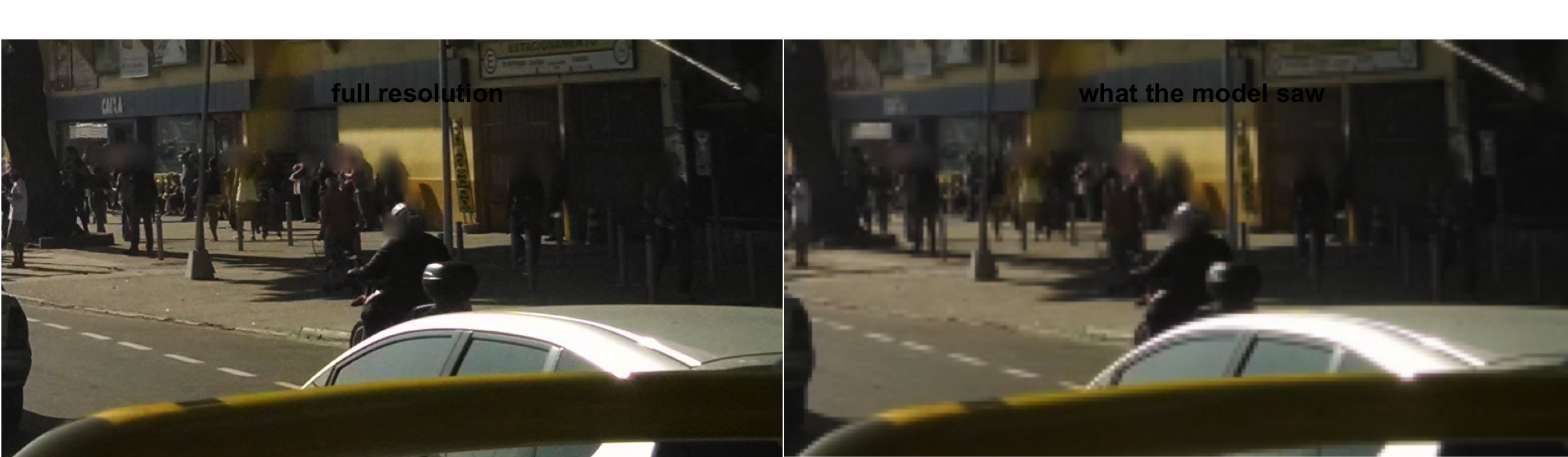
At the model’s resolution, the people on the pavement are blurred into a few blocks of dark cells. You can still tell there is a crowd, because you know what a crowd looks like, but the heads, arms and legs that the model relies on are mostly gone.
Laying out the windows
We want windows of 640 × 640 pixels, the model’s own input size, so that each window reaches the model without being shrunk at all. Neighbouring windows should overlap, so that a person who stands on the boundary between two windows appears whole in at least one of them. We ask for an overlap of at least 20%.
WIN     <- 640L
OVERLAP <- 0.2
Along one dimension of length n, the first window starts at 0 and the last window must end exactly at n. We need enough windows that consecutive starts are no more than WIN * (1 - OVERLAP) pixels apart, and we space them evenly between the first and the last.
window_starts <- function(n, size = WIN, overlap = OVERLAP) {
    k <- ceiling((n - size) / (size * (1 - overlap))) + 1   # number of windows
    round(seq(0, n - size, length.out = k))
}

window_starts(ncol(street))
# [1]    0  432  864 1296 1728 2160 2592
window_starts(nrow(street))
# [1]    0  446  892 1338 1784
Every window is then a combination of a row start and a column start. expand_grid() creates all combinations.
make_windows <- function(r, size = WIN, overlap = OVERLAP) {
    expand_grid(row0 = window_starts(nrow(r), size, overlap),
                col0 = window_starts(ncol(r), size, overlap)) %>%
        mutate(window = row_number())
}

street_windows <- make_windows(street)
street_windows
# # A tibble: 35 x 3
#     row0  col0 window
#    <dbl> <dbl>  <int>
#  1     0     0      1
#  2     0   432      2
#  3     0   864      3
#  4     0  1296      4
#  5     0  1728      5
#  6     0  2160      6
#  7     0  2592      7
#  8   446     0      8
#  9   446   432      9
# 10   446   864     10
# # i 25 more rows
row0 and col0 are the image row and column where each window’s top-left corner sits. To crop a window from the raster, we need its extent in map coordinates. As in the previous post, image rows count down from the top and map y counts up from the bottom, so the window’s top edge, at image row row0, is at map y h - row0.
window_extent <- function(r, row0, col0, size = WIN) {
    ext(col0, col0 + size, nrow(r) - row0 - size, nrow(r) - row0)
}

draw_extent <- function(e, ...) {
    v <- as.vector(e)   # xmin, xmax, ymin, ymax
    rect(v[1], v[3], v[2], v[4], ...)
}
To demonstrate, we pick the window that contains the most of the single pass’s detections, which is on the pavement.
centres <- street_single %>% mutate(cx = (xmin + xmax) / 2, cy = (ymin + ymax) / 2)
one <- street_windows %>%
    mutate(n = map2_int(row0, col0, ~ sum(between(centres$cx, .y, .y + WIN) &
                                          between(centres$cy, .x, .x + WIN)))) %>%
    slice_max(n, n = 1, with_ties = FALSE)
one
# # A tibble: 1 x 4
#    row0  col0 window     n
#   <dbl> <dbl>  <int> <int>
# 1  1338  2592     28     3
With 35 overlapping windows, drawing all their outlines produces an unreadable mesh. A clearer way to see the layout is itself a raster: a coverage raster, in which each cell holds the number of windows that see it. We make a coarse template covering the photograph, turn each window’s extent into a polygon, rasterize it (1 inside the window, 0 outside), and add them up.
coverage <- function(r, windows, res = 8) {
    template <- rast(ext(r), resolution = res, crs = crs(r))
    cover <- init(template, 0)
    for (i in seq_len(nrow(windows))) {
        e <- window_extent(r, windows$row0[i], windows$col0[i])
        cover <- cover + rasterize(as.polygons(e, crs = crs(r)), template, background = 0)
    }
    cover
}

street_cover <- coverage(street, street_windows)
freq(street_cover) %>% mutate(share = count / sum(count))
#   layer value count     share
# 1     1     1 50840 0.4153188
# 2     1     2 56284 0.4597915
# 3     1     4 15288 0.1248897
Only part of the photograph is seen by a single window. The rest lies in the overlap strips, seen twice, or where four windows meet at a corner.
cover_colors <- c("1" = "#FFFFB2", "2" = "#FD8D3C", "3" = "#E31A1C", "4" = "#800026")

plot_coverage <- function(r, cover, main = NULL) {
    plotRGB(r, mar = c(0, 0, if (is.null(main)) 0 else 1.5, 4))
    if (!is.null(main)) title(main, line = 0.2)
    v <- sort(unique(values(cover)))
    plot(cover, add = TRUE, type = "classes", col = cover_colors[as.character(v)],
         alpha = 0.5, plg = list(title = "windows"))
}
plot_coverage(street, street_cover)
draw_extent(window_extent(street, one$row0, one$col0), border = "yellow", lwd = 3)
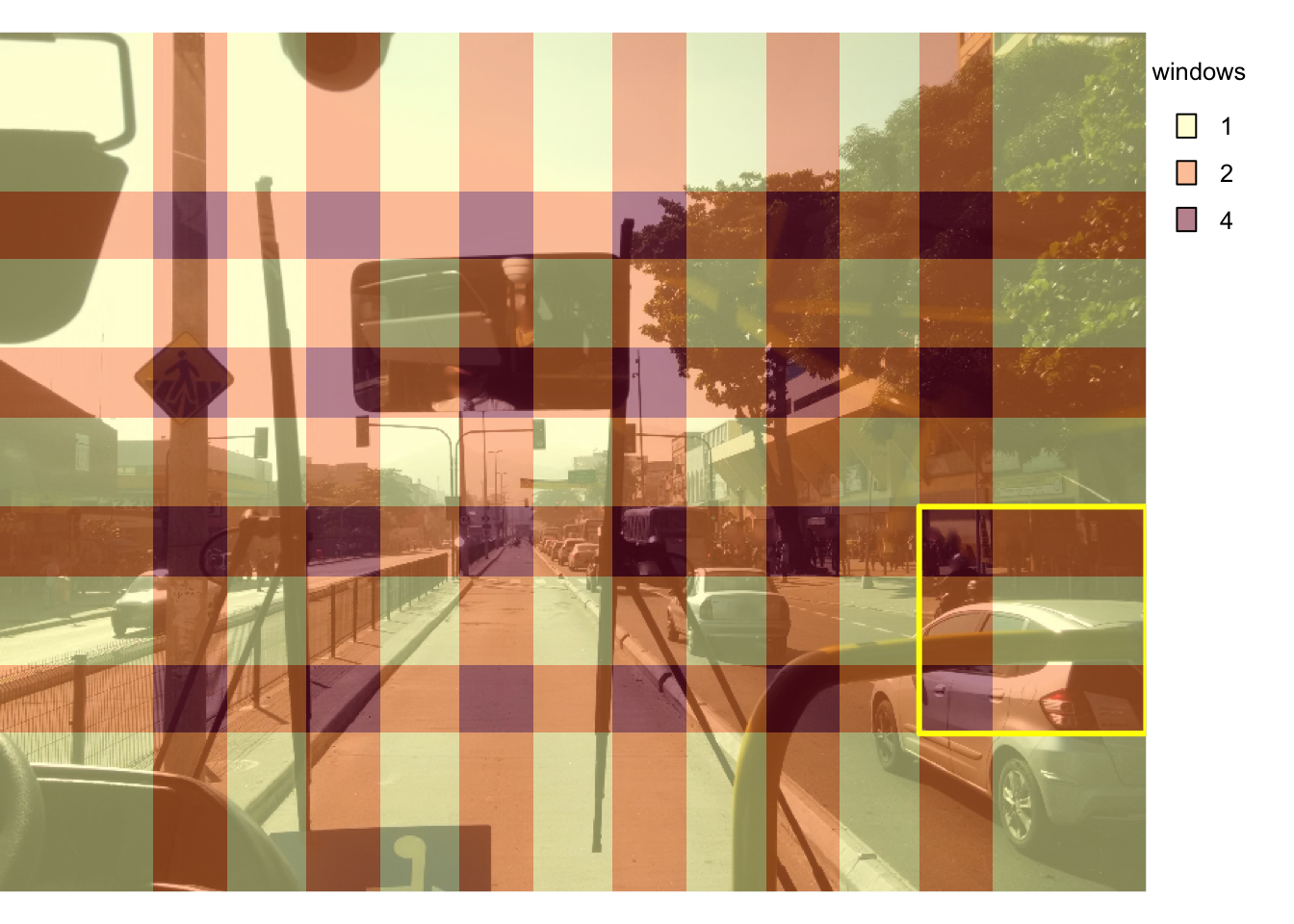
The yellow square is the window we will look at first.
The model will run once for each window, so this approach costs about 35 times as much computation as a single pass.
Detecting in one window
Take the highlighted window. Cropping gives a 640 × 640 raster, and detect_raster() returns its detections in the window’s own pixel coordinates.
one_rast <- crop(street, window_extent(street, one$row0, one$col0))
dim(one_rast)
# [1] 640 640   3

one_dets <- detect_raster(one_rast)
one_dets
# # A tibble: 4 x 7
#     xmin  ymin  xmax  ymax  conf class_id class
#    <dbl> <dbl> <dbl> <dbl> <dbl>    <dbl> <chr>
# 1  41.2  132.  174.   306. 0.832        0 person
# 2   4.45  96.2  59.0  252. 0.776        0 person
# 3 116.   206.  208.   281. 0.539        0 person
# 4 417.    55.7 485.   258. 0.514        0 person
plot_detections(one_rast, one_dets)
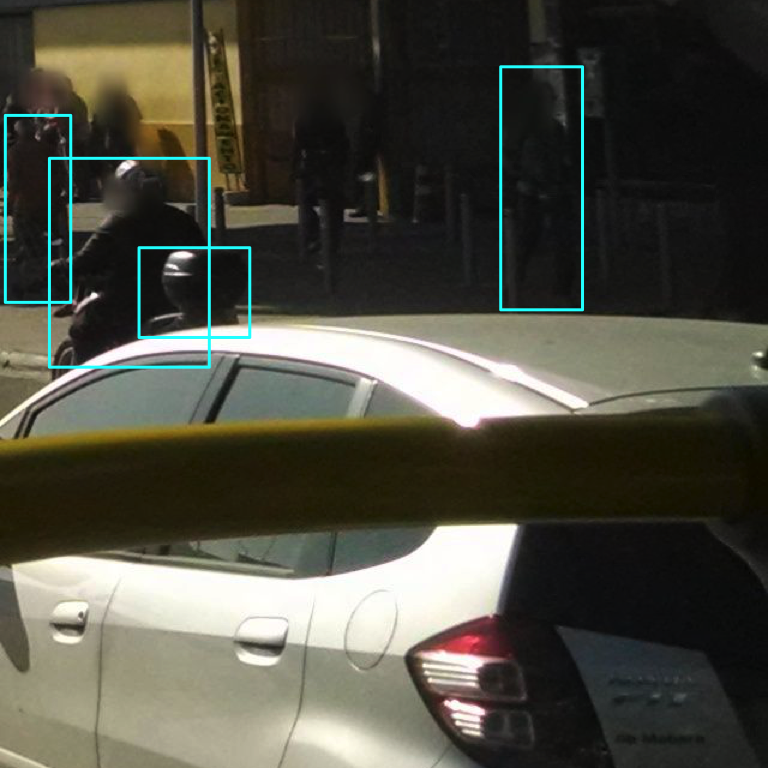
At full resolution, the model finds people that the single pass could not. It is not always right, though. The motorcycle’s rider is a person, which is correct as far as the COCO categories go, but not a pedestrian. And the smallest box, with the lowest confidence, is on the motorcycle’s top case. Keep both in mind: more detail brings more detections, and not all of them are what we want.
To place these boxes on the full photograph, shift them by the window’s position: add col0 to the x coordinates and row0 to the y coordinates.
one_dets %>%
    mutate(xmin = xmin + one$col0, xmax = xmax + one$col0,
           ymin = ymin + one$row0, ymax = ymax + one$row0)
# # A tibble: 4 x 7
#    xmin  ymin  xmax  ymax  conf class_id class
#   <dbl> <dbl> <dbl> <dbl> <dbl>    <dbl> <chr>
# 1 2633. 1470. 2766. 1644. 0.832        0 person
# 2 2596. 1434. 2651. 1590. 0.776        0 person
# 3 2708. 1544. 2800. 1619. 0.539        0 person
# 4 3009. 1394. 3077. 1596. 0.514        0 person
Detecting in every window
The same steps, applied to every row of the windows table with pmap_dfr(), give the detections from every window in photograph coordinates. We also keep the single-pass detections, labelled as window 0. The single pass still has a job to do: a person close to the camera can be larger than a window, and only the single pass sees them whole.
detect_in_windows <- function(r, windows) {
    pmap_dfr(windows, function(row0, col0, window) {
        detect_raster(crop(r, window_extent(r, row0, col0))) %>%
            mutate(xmin = xmin + col0, xmax = xmax + col0,
                   ymin = ymin + row0, ymax = ymax + row0,
                   window = window)
    })
}

street_raw <- bind_rows(
    street_single %>% mutate(window = 0L),
    detect_in_windows(street, street_windows)
)
nrow(street_raw)
# [1] 34
plot_detections(street, street_raw, paste("all windows:", nrow(street_raw), "boxes"))
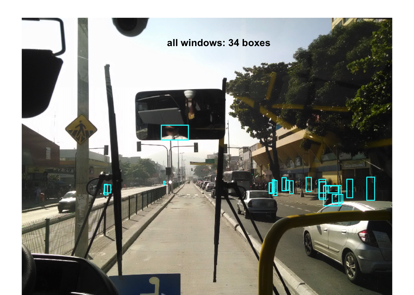
There are 34 boxes, but far fewer people. Because the windows overlap, a person in an overlap zone is detected in two windows, and a person where four windows meet can be detected in four. We need to merge these duplicates into one box per person.
Merging duplicates
Measuring overlap
Two boxes are probably the same person if they overlap a lot. The standard measure of overlap is the intersection over union (IoU): the area the two boxes share, divided by the total area they cover together. It is 1 for identical boxes and 0 for boxes that do not touch.
box_iou <- function(a, b) {
    iw <- pmax(0, pmin(a$xmax, b$xmax) - pmax(a$xmin, b$xmin))   # width of the intersection
    ih <- pmax(0, pmin(a$ymax, b$ymax) - pmax(a$ymin, b$ymin))   # height of the intersection
    inter <- iw * ih
    area_a <- (a$xmax - a$xmin) * (a$ymax - a$ymin)
    area_b <- (b$xmax - b$xmin) * (b$ymax - b$ymin)
    inter / (area_a + area_b - inter)
}
box_iou() compares one box a against any number of boxes b, because pmin() and pmax() work element by element.
toy <- tibble(xmin = c(0, 10, 100), ymin = 0, xmax = c(40, 50, 140), ymax = 100)
box_iou(toy[1, ], toy)   # itself, a shifted copy, a distant box
# [1] 1.0 0.6 0.0
Non-maximum suppression
Non-maximum suppression (NMS) uses IoU to remove duplicates. Sort the boxes by confidence. Keep the most confident box, and discard every remaining box that overlaps it by more than a threshold. Then move to the next most confident box that is still left, and repeat.
nms <- function(dets, overlap_fn = box_iou, thresh = 0.5) {
    dets <- arrange(dets, desc(conf))
    keep <- rep(TRUE, nrow(dets))
    for (i in seq_len(nrow(dets))) {
        if (!keep[i]) next
        rest <- which(keep & seq_len(nrow(dets)) > i)
        if (length(rest) == 0) next
        keep[rest[overlap_fn(dets[i, ], dets[rest, ]) > thresh]] <- FALSE
    }
    dets[keep, ]
}

street_iou <- nms(street_raw)
nrow(street_iou)
# [1] 18
plot_detections(street, street_iou, paste("NMS with IoU:", nrow(street_iou)))
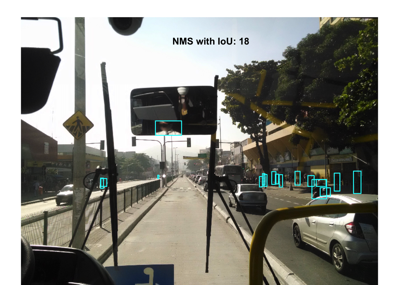
That removed most of the duplicates, but look closely at the people on the pavement. Some of them still have a smaller box inside or overlapping a larger one.
Fragments at window edges
These leftover boxes are fragments. When a window’s edge cuts through a person, the model often still recognises the part it can see, a head and torso without the legs, say, and draws a box around that part only. The same person seen whole in a neighbouring window gets a full-size box. The two boxes overlap a lot, but because one is much smaller than the other, their IoU is low.
toy <- tibble(xmin = c(0, 0), ymin = c(0, 0), xmax = c(40, 40), ymax = c(100, 45))
box_iou(toy[1, ], toy[2, ])   # a full person and the top 45% of the same person
# [1] 0.45
IoU is only 0.45, below the threshold, so NMS keeps both.
One tempting fix is to measure overlap differently: divide the intersection by the area of the smaller box instead of by the union (intersection over smaller, IoS). A fragment lies almost entirely inside the full box, so its IoS is close to 1.
box_ios <- function(a, b) {
    iw <- pmax(0, pmin(a$xmax, b$xmax) - pmax(a$xmin, b$xmin))
    ih <- pmax(0, pmin(a$ymax, b$ymax) - pmax(a$ymin, b$ymin))
    area_a <- (a$xmax - a$xmin) * (a$ymax - a$ymin)
    area_b <- (b$xmax - b$xmin) * (b$ymax - b$ymin)
    iw * ih / pmin(area_a, area_b)
}
box_ios(toy[1, ], toy[2, ])
# [1] 1
The trouble is that IoS cannot tell a fragment from a different person partly hidden behind someone else, which is common on a crowded pavement. Two people walking one behind the other can easily give IoS above 0.5, and one of them would be discarded.
A better fix is to stop fragments from being created in the first place. A box that touches a window’s edge is probably a fragment, unless that edge is also the edge of the photograph. And because the windows overlap, a person cut by one window’s edge should appear whole in a neighbouring window. So we drop every window detection that comes within a few pixels of an inner window edge.
EDGE_MARGIN <- 4   # pixels

drop_edge_boxes <- function(dets, row0, col0, r, size = WIN, margin = EDGE_MARGIN) {
    touches <-
        (dets$xmin < margin        & col0 > 0) |                # left edge, not the photograph's
        (dets$xmax > size - margin & col0 + size < ncol(r)) |   # right edge
        (dets$ymin < margin        & row0 > 0) |                # top edge
        (dets$ymax > size - margin & row0 + size < nrow(r))     # bottom edge
    dets[!touches, ]
}
The check has to happen in the window’s own coordinates, before the boxes are shifted onto the photograph, so it goes inside the loop over windows.
detect_in_windows <- function(r, windows) {
    pmap_dfr(windows, function(row0, col0, window) {
        detect_raster(crop(r, window_extent(r, row0, col0))) %>%
            drop_edge_boxes(row0, col0, r) %>%
            mutate(xmin = xmin + col0, xmax = xmax + col0,
                   ymin = ymin + row0, ymax = ymax + row0,
                   window = window)
    })
}

street_edge <- bind_rows(
    street_single %>% mutate(window = 0L),
    detect_in_windows(street, street_windows)
)
street_final <- nms(street_edge)
nrow(street_final)
# [1] 15
par(mfrow = c(1, 2))
plot_detections(street, street_iou,   paste("NMS with IoU:", nrow(street_iou)))
plot_detections(street, street_final, paste("edge filter, then NMS with IoU:", nrow(street_final)))
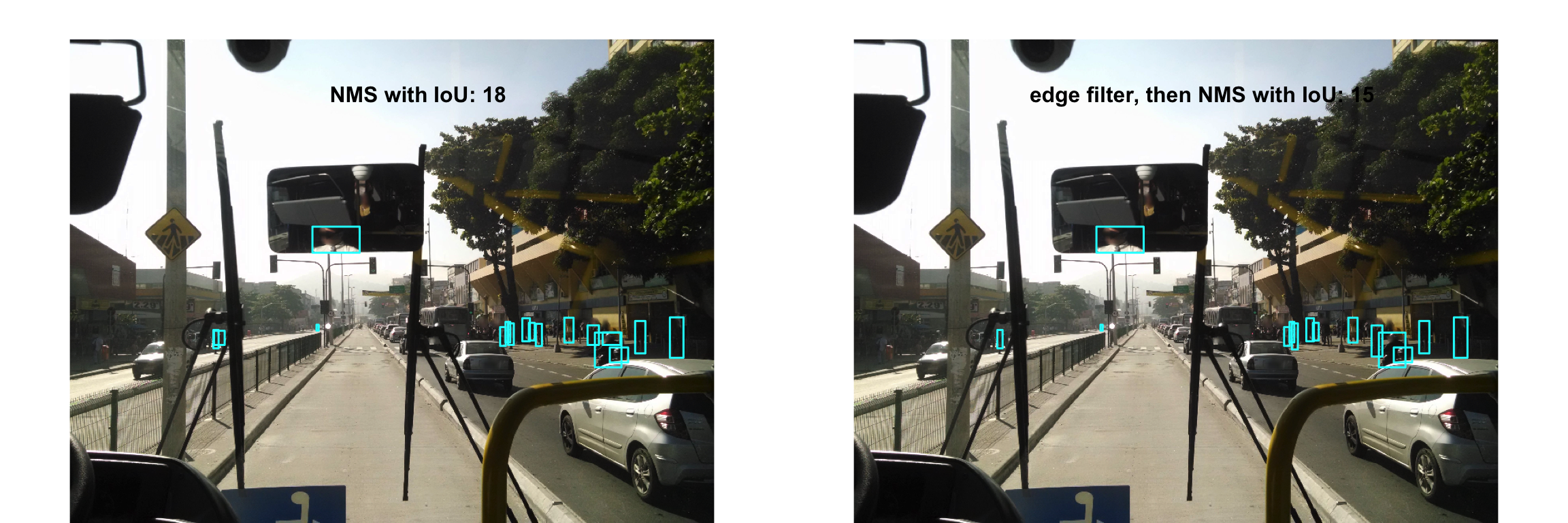
The single pass found 3 pedestrians in this photograph. The windows find 15. Most of the new ones are people on the pavement on the right who were too small to recognise at the single pass’s resolution.
Not every new box is a pedestrian. Look at the rear-view mirror at the top of the photograph: the model has found the bus driver’s reflection. By the model’s standards, that is a correct detection, since there is a person there. For counting pedestrians on the street, it is wrong. More detail helps the model find things, including things you did not want it to find.
Exercise
- Merge
street_rawwithnms(street_raw, overlap_fn = box_ios)instead. Compare the result withstreet_final. Find a place where IoS removed a box that the edge filter kept, and decide which is right. - Change
EDGE_MARGINto 1 and to 20. How do the results change? Why might a box that belongs to a whole person still come within a few pixels of a window’s edge? - The NMS threshold of 0.5 is a convention. Try 0.3 and 0.7. Which duplicates survive, and which real people are removed?
- How would you exclude the reflection in the mirror? Think about what you know about the scene that the model does not.
Putting it together
We collect the steps into one function that takes a photograph and returns its merged pedestrian detections.
detect_pedestrians <- function(r, size = WIN, overlap = OVERLAP) {
    stopifnot("photograph is smaller than one window" = nrow(r) >= size && ncol(r) >= size)
    windows <- make_windows(r, size, overlap)
    bind_rows(
        detect_raster(r) %>% mutate(window = 0L),
        detect_in_windows(r, windows)
    ) %>%
        nms()
}

all.equal(detect_pedestrians(street), street_final)
# [1] TRUE
The stopifnot() guards an assumption that window_starts() makes silently: that the photograph is at least as large as one window. None of the photographs in this collection is smaller than 640 pixels in either dimension, but a function that crops windows from outside the photograph would not tell you so.
Now the beach.
beach_final <- detect_pedestrians(beach)

par(mfrow = c(1, 2))
plot_detections(beach, beach_single, paste("single pass:", nrow(beach_single)))
plot_detections(beach, beach_final,  paste("tiled windows:", nrow(beach_final)))
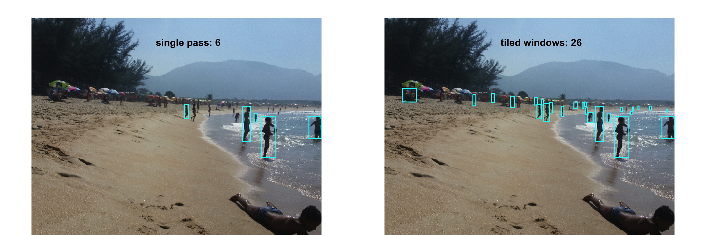
On the beach, the gain is larger still: 6 people in a single pass and 26 with tiled windows. Most of the new detections are people along the shoreline and under the umbrellas in the distance, who are only a few pixels tall at the single pass’s resolution.
Exercise
- Zoom in on the beach photograph and check the new detections by eye. How many are people? How many are something else (an umbrella pole, a post, a shadow)? How many people are still missed?
- Choose a random sample of 30 photographs from
img_files_paths. For each, count pedestrians with a single pass and withdetect_pedestrians(). Plot one count against the other. In which kinds of scenes do the windows help most? Remember to keep the photographs with zero pedestrians. - Time
detect_pedestrians()on one photograph withsystem.time(). How long would the whole collection of 484 photographs take? Is it worth it for your purpose? - Try windows of 1,280 pixels (so the model sees each window at half resolution) and of 320 pixels (where the model enlarges each window). How do the counts and running times change?
- A person close to the camera may be taller than the overlap between windows, or even taller than a window. Which part of our method is responsible for finding them? What happens if you drop the single pass?
detect_raster()keeps onlyperson. Changeclassesto includecar,busandtruck. What happens to a large vehicle close to the camera, which is cut by several windows? Does the edge filter handle it?
Conclusion
A single pass through the model shrinks the photograph to fit the model, and small, distant pedestrians shrink with it until there is nothing left to recognise. Tiled windows let the model see every part of the photograph at full resolution, at the cost of running the model many times and then having to reconcile its answers.
That reconciliation is where most of the work lies. Overlapping windows produce duplicates, and windows that cut through people produce fragments. Non-maximum suppression removes the duplicates. Dropping boxes that touch an inner window edge removes most of the fragments, as long as the windows overlap enough for every person to appear whole somewhere.
More detections are not automatically better detections. The same resolution that reveals distant pedestrians also reveals reflections, posters and shapes that only resemble people. The counts from tiled windows are a better starting point than the counts from a single pass, but they are still a starting point for human review, not a finished count.
Nikhil Kaza
Professor
My research interests include urbanization patterns, local energy policy and equity