Object Detection with YOLO26 and Torch
Introduction
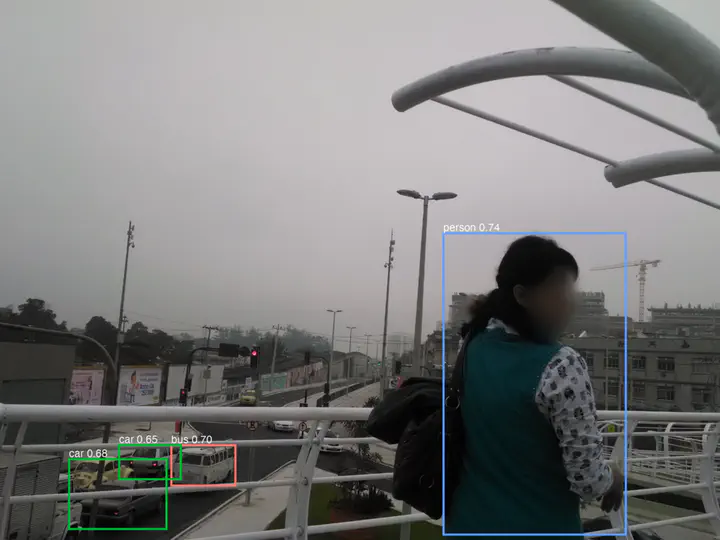
In an earlier post, we used a pre-trained YOLO model from R by reaching into Python with reticulate: import torch and ultralytics, hand a conda environment to use_condaenv(), and call the model as if it were an R object. In this post, I want to examine how we can dispense with the Python requirement. The objective is still the same: take an image (a raster) and see if you can detect objects such as cars, persons and bicycles in the image and locate them. Some elements are repeated from the previous post for the sake of completeness.
Object detection often uses deep learning, though other computer vision tools are occasionally used. Deep learning is a technique that uses neural networks that are ‘deep’ (multiple layers) as opposed to shallow, single-layer networks. Neural networks are a type of computer model inspired by how the human brain works; they learn patterns from data and use that knowledge to make predictions or recognise things.
They require an enormous amount of training data. One of the most widely used datasets for training these models is the COCO dataset (Common Objects in Context), which contains thousands of labelled images featuring everyday scenes with people, vehicles, animals, and more. Because training a neural network from scratch requires a lot of data and computing power, we often use pretrained models (models that have already been trained on datasets like COCO) and then fine-tune them for specific tasks or environments. This makes it easier and faster to apply object detection in real-world settings, including urban planning, without needing to build everything from the ground up. In many instances, you may even skip the fine-tuning step and go straight to inference with an existing model.
This post shows the procedure for doing the entire inference step in R with a model that is already trained. It relies on the R torch package, which binds directly to libtorch (the C++ library that PyTorch itself is built on). Once a model has been exported to the TorchScript format, torch::jit_load() reads it directly.
The price of dropping Python is that the model no longer prepares images for you. Everything that ultralytics did quietly (resizing, padding, rearranging pixel values into the layout the network expects, translating boxes back onto the photograph) is now our job. That turns out to be a good way to learn how raster data works. The post proceeds in the following order:
- Treat a single photograph as a raster: its grid, bands, pixel values and coordinate system.
- Transform that one photograph, step by step, into the input the model expects.
- Run the model, read its raw output, and draw the bounding boxes.
- Use the boxes to cut the detected objects back out of the raster.
- Wrap the steps into functions, and test them on photographs that do not fit the assumptions we made along the way.
- Run the functions across many photographs.
Because Ultralytics produces Python models, we first need to export the model to the TorchScript format. TorchScript compiles a PyTorch model into a static graph that can run independently of the Python runtime. This is the only step that needs Python, and it only needs to happen once. You can download the exported copy. Save it in your InputData folder. I show the export command only for the sake of completeness.
pip install ultralytics
yolo export model=yolo26s.pt format=torchscript imgsz=640 nms=False
The nms=False matters. YOLO26 can be exported in two forms. The end-to-end form removes duplicate boxes inside the model and returns at most 300 final detections, each with six numbers: a 1 × 300 × 6 tensor. The other form returns every raw candidate box for 80 classes: a 1 × 84 × 8400 tensor, which then needs a separate duplicate-removal step called non-maximum suppression (NMS). Which form you get by default depends on the version of Ultralytics. Older versions exported the end-to-end form by default, while newer ones export the raw form unless you set nms=False. Setting it explicitly gives the end-to-end form, which is what this post expects, regardless of version.
yolo26s variant. Swap in yolo26m/l/x for more accuracy at the cost of speed, using the same export command above.
Setup
You might need a few packages that are unusual. torch::install_torch() downloads the libtorch binaries for your platform and only needs to be run once.
install.packages(c("torch", "terra", "exiftoolr"))
torch::install_torch() # downloads libtorch itself, once
library(torch)
library(terra)
library(tidyverse)
library(exiftoolr)
library(here)
All the image handling in this post is done with terra. It is usually used for satellite imagery and elevation models, but a photograph is also a raster, and every operation we need (reading, resizing, padding, cropping, summarising) is a standard raster operation. The only thing to be mindful of, is that terra’s spatRaster expects a geographic coordinate system and an extent that is usually tied to earth. But as we discussed before, georasters are not the only types of rasters.
Data
We’ll use the same street-level images from Rio de Janeiro, Brazil as the earlier post, collected through Kartaview. See that post’s Data section for a fuller discussion of the imagery. Download the images and unzip them into your InputData folder.
img_files_paths <- here("InputData", "geotagged") %>%
              list.files(full.names = TRUE, pattern = "\\.jpg$")
length(img_files_paths)
# [1] 484
Say I want to examine some random images instead of viewing the entire 484 image set. I can use a simple for loop or the more elegant map. I will demonstrate both:
set.seed(123)

img_sample_paths <- sample(img_files_paths, 10)

list_rasters_loop <- list() # initialise a list

for (i in 1:length(img_sample_paths)){
list_rasters_loop[[i]] <- rast(img_sample_paths[i])
}

list_rasters_map <- map(img_sample_paths, rast)

# rast() reads each image as a raster.
all.equal(list_rasters_loop,list_rasters_map)
# [1] TRUE
opar <- par() # save par settings
par(mfrow = c(2, 5)) # arrange the plots in 2 rows and 5 columns
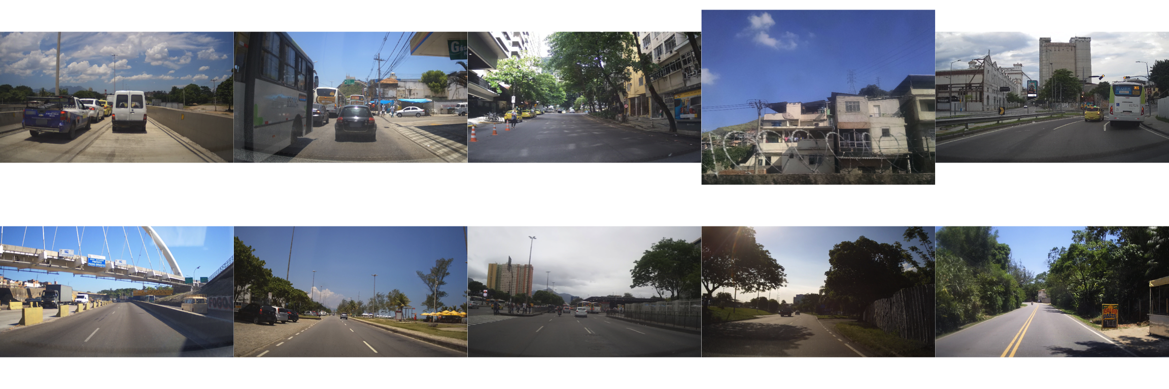
walk(list_rasters_map, plotRGB) # walk() is map() for functions called for their side effects, like plotting
par(opar) # reset to original settings
Note the variation in lighting conditions, angles, zoom levels, focus and occlusions. This is typical of street-level imagery and can pose challenges for object detection models. Also note the differences in urban settings such as highway, commercial corridor, vegetation cover etc.
In addition to data within the images, it is useful to look at the metadata associated with the images. In the case of images, metadata can include details such as the date and time the photo was taken, camera type, the camera settings used, and the geographic location (latitude and longitude) where the image was captured. EXIF (Exchangeable Image File Format) is a standard that stores metadata within image files. This information is automatically recorded by most digital cameras and smartphones and we can use the exiftoolr package to extract it. exiftoolr requires exiftool to be installed on your computer. You can find instructions here or uncomment the appropriate line in the code.
# install_exiftool() # Uncomment this line if you don't have exiftool installed already.

img_metadata <- img_files_paths %>%
                exif_read(tags = c("FileName", "ImageWidth", "ImageHeight", "Megapixels",
                                   "GPSLatitude", "GPSLongitude")) %>%
                as_tibble() %>%
                dplyr::select(-SourceFile)

head(img_metadata)
# # A tibble: 6 x 6
#   FileName            ImageWidth ImageHeight Megapixels GPSLatitude GPSLongitude
#   <chr>                    <int>       <int>      <dbl>       <dbl>        <dbl>
# 1 1318411189__364540~       3232        2424       7.83       -22.9        -43.3
# 2 1318412961__364542~       3232        2424       7.83       -22.9        -43.3
# 3 1318413125__364540~       3232        2424       7.83       -22.9        -43.3
# 4 1318413497__364542~       3232        2424       7.83       -22.8        -43.3
# 5 1318413949__364542~       3232        2424       7.83       -22.8        -43.3
# 6 1318414553__364542~       3232        2424       7.83       -22.8        -43.3
Since we read the metadata for every image rather than just the sample, we can check an assumption that is easy to make. that all the photographs are the same size.
img_metadata %>% count(ImageWidth, ImageHeight, sort = TRUE)
# # A tibble: 10 x 3
#    ImageWidth ImageHeight     n
#         <int>       <int> <int>
#  1       3072        1728   387
#  2       3232        2424    36
#  3       1920        1080    29
#  4       3264        1836    14
#  5       2340        4160     7
#  6       3984        2988     4
#  7       4032        3024     4
#  8       3264        2448     1
#  9       3840        2160     1
# 10       5312        2988     1
They are not. Most images are 3,072 × 1,728 pixels, but there are several other sizes, and a handful of them are taller than they are wide (portrait orientation). We will build the whole pipeline on one landscape photograph, and these other photographs will test it later.
Exercise
- Visualise the locations of all images. Note any patterns you see in the spatial distribution of images. Does the spatial distribution influence any conclusions you might draw about the urban environment?
- Notice that this particular dataset does not have the heading of the camera. Or the lens height. Or the yaw. Or any number of other settings that affect the captured image. How might these absences influence your analysis downstream?
A photograph is a raster
A digital photograph is a raster: a rectangular grid of cells (pixels), each holding numbers. The post on drone imagery discusses the several ways to think about rasters. Here we look at one street-level photograph through that lens. We will use the same photograph for the next several sections.
example_path <- img_files_paths[str_detect(img_files_paths, "1318411189")]
basename(example_path)
# [1] "1318411189__3645401_74b21_60c0ec1f7c728.jpg"

(example_rast <- rast(example_path))
# class       : SpatRaster
# size        : 2424, 3232, 3  (nrow, ncol, nlyr)
# resolution  : 1, 1  (x, y)
# extent      : 0, 3232, 0, 2424  (xmin, xmax, ymin, ymax)
# coord. ref. :
# source      : 1318411189__3645401_74b21_60c0ec1f7c728.jpg
# colors rgb  : 1, 2, 3
# names       : 1318411189~c1f7c728_1, 1318411189~c1f7c728_2, 1318411189~c1f7c728_3
terra reads the JPEG as a SpatRaster, the same kind of object it would produce for a satellite image or a digital elevation model. The printout tells us most of what we need:
- size: 2,424 rows, 3,232 columns and 3 layers. That is 7,834,368 pixels in each layer.
- layers (bands): a colour photograph has three bands: red, green and blue. Every colour you see is some mix of these three values at that pixel.
- resolution: 1 × 1. There is no real-world unit here; one cell is one pixel.
- extent: 0 to 3,232 in x, 0 to 2,424 in y. Again, these are pixel units, not metres.
- coord. ref.: empty. A photograph taken from a car is not georeferenced. Only the camera location is known (from the EXIF data); the pixels themselves have no map coordinates. Contrast this with an orthomosaic from a drone, where every pixel can be placed on a map.
When the three bands are combined as red, green and blue, we get the photograph.
names(example_rast) <- c("red", "green", "blue")
plotRGB(example_rast)
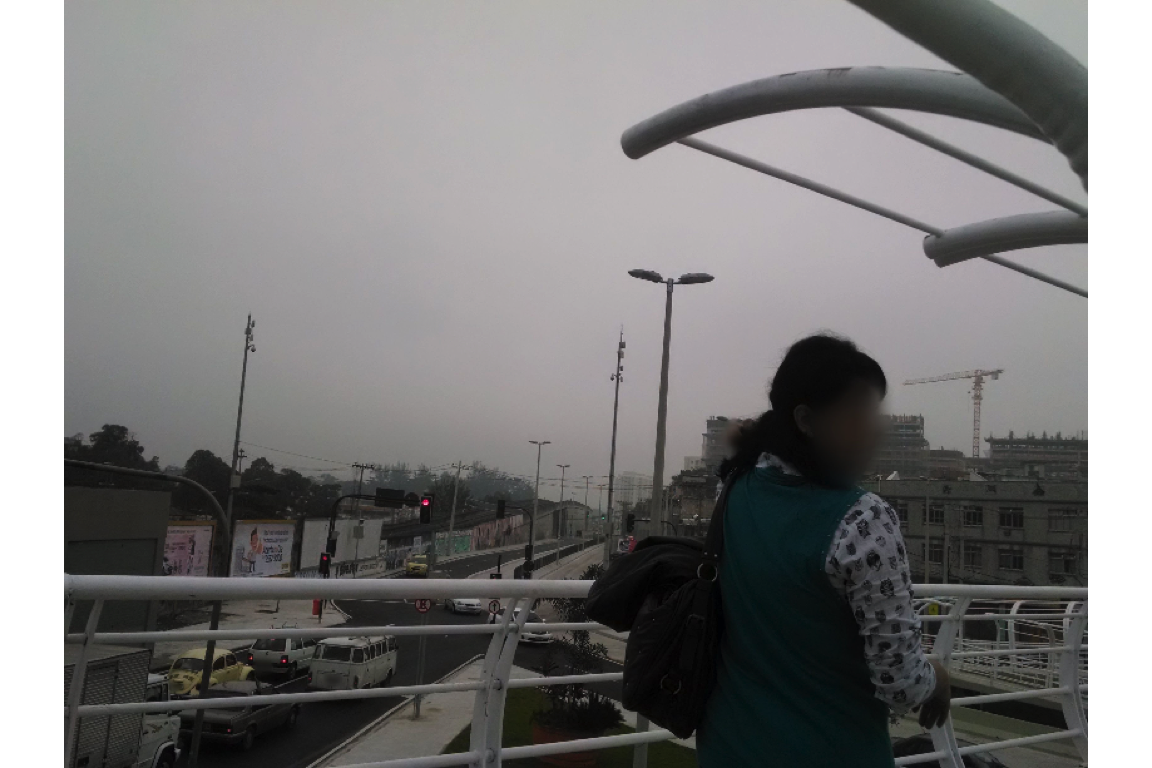
Each pixel holds three integers from 0 to 255 (2^8 - binary 8 bit), one byte per band.
global(example_rast, c("min", "max", "mean"))
#       min max     mean
# red     0 255 121.9481
# green   0 255 121.4019
# blue    0 233 121.0659
The three means are almost the same. This is a foggy day, and most of the photograph (sky, concrete, railings) is some shade of grey, which is what you get when red, green and blue are roughly equal. The distributions of values in the three bands show this directly. We sample a regular grid of pixels rather than use all 7,834,368 of them.
band_colors <- c(red = "red", green = "green3", blue = "blue")

spatSample(example_rast, 50000, method = "regular") %>%
    pivot_longer(everything(), names_to = "band") %>%
    ggplot(aes(x = value, colour = band)) +
    geom_density() +
    scale_colour_manual(values = band_colors, guide='none') +
    labs(x = "pixel value (0-255)", y = "density") +
    theme_minimal()
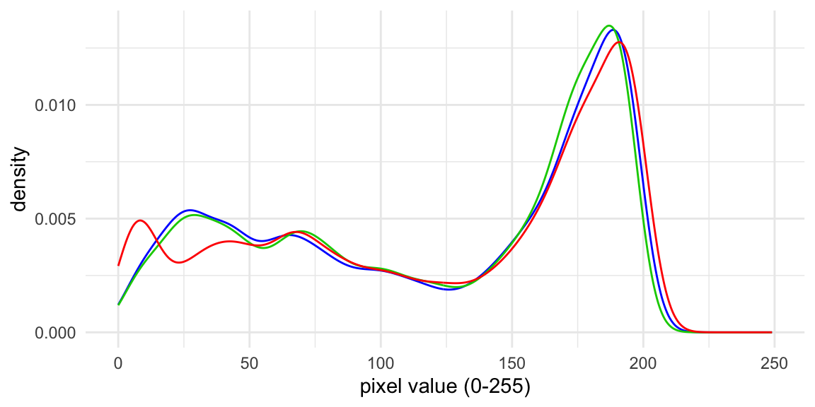
The large peak near 190 is the sky. Because the bands overlap so closely, plotting each band on its own would show three near-identical greyscale pictures. The colour in this photograph lives in the small differences between bands, and rasters make those easy to compute. Arithmetic on rasters works cell by cell, so subtracting one band from another gives a new raster.
red_minus_blue <- example_rast$red - example_rast$blue
global(red_minus_blue, quantile, probs = c(0.01, 0.5, 0.99))
#     X1. X50. X99.
# red -29    1   17

# saturate the colour scale at +/- 60 so small differences stay visible
plot(clamp(red_minus_blue, -60, 60), col = hcl.colors(100, "Blue-Red 3"),
     range = c(-60, 60), axes = FALSE, mar = c(0.5, 0.5, 0.5, 4))
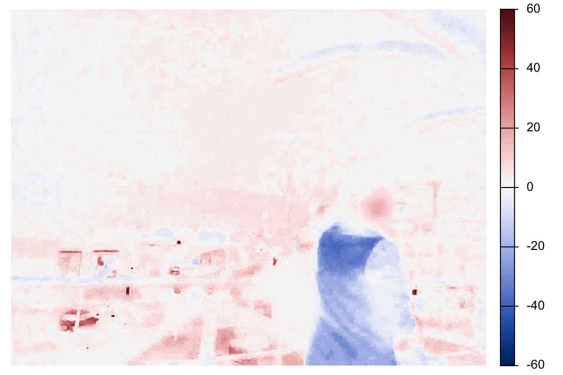
Grey pixels, where red and blue are equal, are white. The woman’s teal top is strongly blue. The traffic signals, the brake lights, her face and the yellow Beetle in the lower left are red. The median difference is only 1, and 98% of pixels lie between -29 and 17.
Pixel coordinates and map coordinates
This is most important detail in this post, so it is worth paying attention to. There are two ways to refer to a location in this raster.
- Row and column (image convention). Row 1 is the top of the photograph, and rows increase downward. This is how cameras, image editors and object detection models count pixels.
- x and y (map convention). y = 0 is the bottom of the extent, and y increases upward, as it does on a map or a
ggplot.
top_left <- cellFromRowCol(example_rast, row = 1, col = 1)
example_rast[top_left]        # pixel values of the top-left pixel
#   red green blue
# 1 176   172  173
xyFromCell(example_rast, top_left)   # its x,y coordinates
#        x      y
# [1,] 0.5 2423.5
The top-left pixel has row 1 but a y coordinate of 2,423.5, near the top of the y axis. Note that .5 refers to the fact that terra puts the pixel coordinate at the center of the pixel rather than at the edge. In general, for a photograph with height h, an image row coordinate y_img corresponds to a map y coordinate of h - y_img. We will need this conversion every time we draw or crop a bounding box, because the model reports boxes in image coordinates rather than map coordinates.
Rasters as arrays
A raster with bands is also a three-dimensional array. terra can give it to us as rows × columns × bands.
example_arr <- as.array(example_rast)
dim(example_arr)
# [1] 2424 3232    3
example_arr[1, 1, ]   # row 1, column 1, all three bands
# [1] 176 172 173
terra also numbers the cells of a raster with a single index. The numbering runs along the first row from left to right, then along the second row, and so on.
cellFromRowCol(example_rast, row = 1, col = 1:3)   # first three cells of row 1
# [1] 1 2 3
cellFromRowCol(example_rast, row = 2, col = 1)     # first cell of row 2 is ncol+1
# [1] 3233
values() returns the pixel values as a matrix with one row per cell, in this order, and one column per band.
head(values(example_rast))
#      red green blue
# [1,] 176   172  173
# [2,] 175   171  172
# [3,] 174   170  171
# [4,] 174   170  171
# [5,] 174   170  171
# [6,] 174   170  171
Keep this row-by-row order in mind. R fills arrays and matrices the other way, column by column, and mixing up the two is an easy mistake to make. We will come back to it.
Exercise
- Pick a pixel in the sky and a pixel on the road. Use
cellFromRowCol()and indexing to extract their values. Which band distinguishes them most? - Compute the mean of the three bands (
mean(example_rast)) and plot it. What have you created? Why might a model that only saw this single band do worse at telling a red bus from a green one? - Use
global()andmap_dbl()to compute the mean brightness of each raster inlist_rasters_map. Do the darker photographs match the ones you picked out by eye?
A digression on vectors, matrices and tensors
Before we hand the photograph to the model, it is worth being precise about the containers that numbers live in. The model’s input requirements, and the easiest mistakes to make when meeting them, are both about how numbers are arranged rather than what they are.
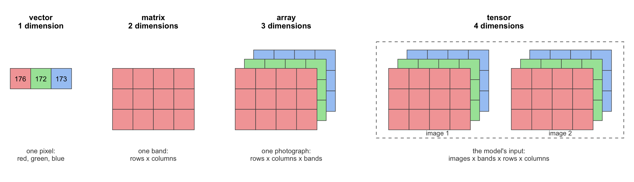
The diagram shows the four containers we will use, each built from the one before it by adding a dimension. The tensor is drawn with two images to make the images dimension visible. In this post, the model’s input will be a batch of one image.
Vectors
A vector is a sequence of numbers with one dimension. The three band values of a single pixel are a vector.
pixel <- c(176, 172, 173)
length(pixel)
# [1] 3
dim(pixel)   # a plain vector has no dim attribute
# NULL
Matrices
A matrix is a vector with a dim attribute of length 2: rows and columns. The numbers are stored in one long sequence, and the dim attribute says how to lay them out.
x <- 1:12
dim(x) <- c(3, 4)   # the same 12 numbers, now as 3 rows and 4 columns
x
#      [,1] [,2] [,3] [,4]
# [1,]    1    4    7   10
# [2,]    2    5    8   11
# [3,]    3    6    9   12
Notice the order. R fills a matrix column by column: 1, 2, 3 go down the first column before 4 starts the second. To fill row by row, you have to ask for it.
matrix(1:12, nrow = 3, byrow = TRUE)
#      [,1] [,2] [,3] [,4]
# [1,]    1    2    3    4
# [2,]    5    6    7    8
# [3,]    9   10   11   12
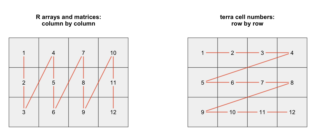
The line in each grid follows the order in which the numbers are stored. Row by row is the order terra uses to number cells, which is why the difference matters. A single band of a raster is a matrix of rows × columns.
red_matrix <- as.matrix(example_rast$red, wide = TRUE)
dim(red_matrix)
# [1] 2424 3232
Arrays
Arrays extend matrices to any number of dimensions. A colour photograph is a 3-dimensional array: rows × columns × bands. Here is a tiny 2 × 3 pixel “photograph” with three bands, small enough to print.
tiny <- array(seq(10, 180, by = 10), dim = c(2, 3, 3))
tiny
# , , 1
#
#      [,1] [,2] [,3]
# [1,]   10   30   50
# [2,]   20   40   60
#
# , , 2
#
#      [,1] [,2] [,3]
# [1,]   70   90  110
# [2,]   80  100  120
#
# , , 3
#
#      [,1] [,2] [,3]
# [1,]  130  150  170
# [2,]  140  160  180
Each index selects along one dimension, and leaving an index empty keeps everything along that dimension.
tiny[, , 1]    # the first band: a 2 x 3 matrix
#      [,1] [,2] [,3]
# [1,]   10   30   50
# [2,]   20   40   60
tiny[1, 2, ]   # the pixel in row 1, column 2: a vector of 3 band values
# [1]  30  90 150
The order of the dimensions is only a convention. aperm() (array permutation) reorders the dimensions and moves the numbers along with them, so every value stays attached to the same pixel and band. Here we put bands first.
tiny_chw <- aperm(tiny, c(3, 1, 2))   # bands, rows, columns
dim(tiny_chw)
# [1] 3 2 3
tiny_chw[, 1, 2]   # the same pixel as tiny[1, 2, ]
# [1]  30  90 150
Changing the dim attribute is a very different operation. It keeps the numbers in their stored order and only changes how they are laid out, so the result has the right shape and the wrong contents.
tiny_wrong <- tiny
dim(tiny_wrong) <- c(3, 2, 3)   # right shape, numbers not moved
tiny_wrong[, 1, 2]              # not the pixel we wanted
# [1] 70 80 90
identical(tiny_wrong, tiny_chw)
# [1] FALSE
When you need to reorder the dimensions of an array, use aperm(). Resetting dim() or passing the values to array() will give you a result of the right shape, with no error, whose numbers have been scrambled.
Tensors
A tensor is torch’s version of an array: a grid of numbers with any number of dimensions. There are a few practical differences from an R array.
- A tensor is stored and managed by
libtorch, outside R, and can be moved to a graphics card (GPU) for faster computation. Itsdevicesays where it is. - Every tensor has a single numeric type, its
dtype. R stores numbers as 8-byte doubles by default. Models usually expect 4-byte floats (float32), which halves the memory. - Operations are usually called as methods with
$, for examplex$shapeorx$div(255). - Image models conventionally put the channels (bands) first, and expect one more dimension in front for the number of images: images × channels × rows × columns. A single photograph is a batch of one image.
tiny_tensor <- torch_tensor(tiny_chw)
tiny_tensor$shape
# [1] 3 2 3
tiny_tensor$dtype
# torch_Float
tiny_tensor$device
# torch_device(type='cpu')
unsqueeze() adds a dimension of size 1 at the position you give it, and squeeze() removes one. This is how we turn one image into a batch of one.
tiny_batch <- tiny_tensor$unsqueeze(1)
tiny_batch$shape
# [1] 1 3 2 3
tiny_batch$squeeze(1)$shape
# [1] 3 2 3
Indexing works as it does for R arrays. In Python, PyTorch counts positions from 0. The R torch package follows R and counts from 1.
tiny_batch[1, , 1, 2]   # image 1, all bands, row 1, column 2
# torch_tensor
#   30
#   90
#  150
# [ CPUFloatType{3} ]
as.array() converts a tensor back into an R array.
dim(as.array(tiny_batch))
# [1] 1 3 2 3
To summarise the containers we will meet in the rest of the post:
| Object | Dimensions | In this post |
|---|---|---|
| vector | 1 | the band values of one pixel |
| matrix | 2 | one band of the photograph (rows × columns) |
| array | 3 | the photograph (rows × columns × bands) |
| tensor | 4 | the model’s input (images × bands × rows × columns) |
Exercise
- Use
aperm()to turntiny_chwback into rows × columns × bands. Check that the result isidentical()totiny. - What does
torch_tensor(1:5)$dtypereturn? Why does it differ fromtiny_tensor$dtype? example_arrholds 23,503,104 numbers. Useobject.size()to find how much memory it takes as an R array. How much would the same numbers take as afloat32tensor?
Object detection with the model
Now load the model.
model <- here("InputData", "yolo26s.torchscript") %>% jit_load()
The input to the model is a tensor: a multi-dimensional array of numbers in a specific shape. What happens if we simply give it our photograph?
attempt <- example_rast %>% model %>% try(silent =TRUE)
conditionMessage(attr(attempt, "condition"))
# [1] "Unsupported type"
Normally an error stops R, and when knitting a document it stops the whole render. try() runs an expression and, if it fails, catches the error instead of stopping. The script then carries on.
- If the expression succeeds,
try()returns its value as usual. - If it fails,
try()returns an object of class"try-error". The original error is stored in its"condition"attribute, andconditionMessage()extracts the message from it. silent = TRUEstopstry()from also printing the error to the console.
We use try() here because we expect these calls to fail and want to look at why. Don’t wrap working code in try() to make errors go away. A caught error is still an error.
The model does not know what a SpatRaster is. So let’s convert the photograph’s array into a tensor at its full size. (Step 3 below explains this conversion.)
full_size <- torch_tensor(aperm(as.array(example_rast), c(3, 1, 2)))$unsqueeze(1)
full_size$shape
# [1]    1    3 2424 3232

attempt <- try(model(full_size), silent = TRUE)
conditionMessage(attr(attempt, "condition")) %>% str_extract("^[^\n]*")   # first line of a long message
# [1] "The following operation failed in the TorchScript interpreter."
It fails again, this time from inside the network. When we exported the model with imgsz=640, it was fixed to one input shape: 1 image × 3 bands × 640 rows × 640 columns. Any other shape fails. So we need to turn a 3,232 × 2,424 photograph into a 640 × 640 raster without distorting it. There are three steps: resample, pad, and rearrange.
IMG_SIZE    <- 640L
PAD_VALUE   <- 114         # grey; Ultralytics' own padding value
CONF_THRESH <- 0.5
Step 1: Resample
Resampling changes the number of pixels in a raster. Going from 3,232 columns to 640 means each new pixel summarises roughly a 5 × 5 block of the original ones. We lose detail, and small or distant objects may disappear. This is one reason why detection models are less reliable for things far from the camera.
We want to shrink the photograph so that its longer side becomes 640 pixels, and shrink the other side by the same factor, so that a car keeps its shape. For this photograph the width is the longer side.
w <- ncol(example_rast)
h <- nrow(example_rast)

scale <- IMG_SIZE / w      # width is the longer side of this photograph
new_w <- round(w * scale)
new_h <- round(h * scale)
c(scale = scale, new_w = new_w, new_h = new_h)
#       scale       new_w       new_h
#   0.1980198 640.0000000 480.0000000
In terra, resampling works by describing the raster you want (a template) and asking resample() to fill it from the original. The template covers the same extent as the photograph but has only 640 × 480 cells.
ext(example_rast) <- ext(0, w, 0, h)

template <- rast(nrows = new_h, ncols = new_w, nlyrs = 3,
                 extent = ext(example_rast), crs = crs(example_rast))
resized <- resample(example_rast, template, method = "average")
resized
# class       : SpatRaster
# size        : 480, 640, 3  (nrow, ncol, nlyr)
# resolution  : 5.05, 5.05  (x, y)
# extent      : 0, 3232, 0, 2424  (xmin, xmax, ymin, ymax)
# coord. ref. :
# source(s)   : memory
# names       :        red,      green,       blue
# min values  :          0,   0.580433,   0.537202
# max values  : 237.533478, 198.148117, 201.772278
Two details matter here. First, the extent. terra reports an extent of 0 to 3,232 by 0 to 2,424, but a JPEG does not actually store one. terra makes it up, and GDAL, which does the resampling, refuses to work on a file with no extent. Setting the extent explicitly with ext() is enough to satisfy it. Second, the method. With "average", each new cell is the mean of the original cells it covers, which is the natural choice when shrinking an image. "near" would pick a single original pixel instead, and "bilinear" would interpolate from the four nearest. Each gives slightly different pixel values, and so slightly different detections.
Notice that the resolution is now about 5 × 5: each new cell is about 5 original pixels wide. The extent has not changed, only the number of cells covering it.
Step 2: Pad
The resized photograph is 640 × 480, not square. We place it in the middle of a 640 × 640 grey canvas, leaving an equal band of padding at the top and bottom. This is called letterboxing, by analogy with the black bars added to widescreen video on an old square TV. The alternative, stretching the photograph to 640 × 640, would distort every object in it.
In raster terms, padding means extending a raster to a larger extent and filling the new cells with a constant. First we work out where the photograph should sit, in pixels from the top-left corner of the canvas.
left <- (IMG_SIZE - new_w) %/% 2L
top  <- (IMG_SIZE - new_h) %/% 2L
c(left = left, top = top)
# left  top
#    0   80
Then we move the resized raster to that position by giving it a new extent, one unit per cell. The photograph starts top rows down from the top of the canvas. In map coordinates, where y counts up from the bottom, that puts its upper edge at IMG_SIZE - top and its lower edge at IMG_SIZE - top - new_h. This is the image-to-map conversion from earlier, applied to a whole raster.
ext(resized) <- ext(left, left + new_w, IMG_SIZE - top - new_h, IMG_SIZE - top)

padded <- extend(resized, ext(0, IMG_SIZE, 0, IMG_SIZE), fill = PAD_VALUE)
padded
# class       : SpatRaster
# size        : 640, 640, 3  (nrow, ncol, nlyr)
# resolution  : 1, 1  (x, y)
# extent      : 0, 640, 0, 640  (xmin, xmax, ymin, ymax)
# coord. ref. :
# source(s)   : memory
# names       :        red,      green,       blue
# min values  :          0,   0.580433,   0.537202
# max values  : 237.533478, 198.148117, 201.772278
plotRGB(padded)
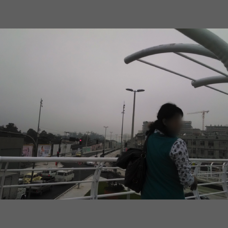
This is what the model will see. Hold on to scale, left and top. Every box the model returns will be in the coordinates of this padded 640 × 640 image, and we will need these three numbers to map the boxes back onto the original photograph.
Step 3: Rearrange into a tensor
The model wants the values as a 4-dimensional array ordered batch × channel × height × width, with values scaled from 0–255 to 0–1. We already know that as.array() gives us height × width × channel. So we move the channel dimension to the front with aperm(), divide by 255, and add a batch dimension of size 1.
padded_arr <- as.array(padded)
dim(padded_arr)                  # height, width, channel
# [1] 640 640   3

chw <- aperm(padded_arr, c(3, 1, 2))
dim(chw)                         # channel, height, width
# [1]   3 640 640

x <- torch_tensor(chw, dtype = torch_float32())$div(255)$unsqueeze(1)
x$shape                          # batch, channel, height, width
# [1]   1   3 640 640
A quick check that the padding ended up where we think it is. Row 80 (the last padded row) should be grey (114/255 ≈ 0.447) in all three bands, and row 81 should be the first row of the photograph.
x[1, , top, 1]
# torch_tensor
#  0.4471
#  0.4471
#  0.4471
# [ CPUFloatType{3} ]
x[1, , top + 1, 1]
# torch_tensor
#  0.6818
#  0.6662
#  0.6702
# [ CPUFloatType{3} ]
Getting the order of values wrong does not produce an error. Suppose that instead of as.array(), we took the matrix from values() and poured it into an array of the right size. values() lists cells row by row, but array() fills column by column, so every row of the photograph ends up as a column.
transposed <- array(values(padded), dim = c(IMG_SIZE, IMG_SIZE, 3))
dim(transposed)
# [1] 640 640   3
par(mfrow = c(1, 2))
plotRGB(padded, main = "correct")
plotRGB(rast(transposed), main = "transposed")
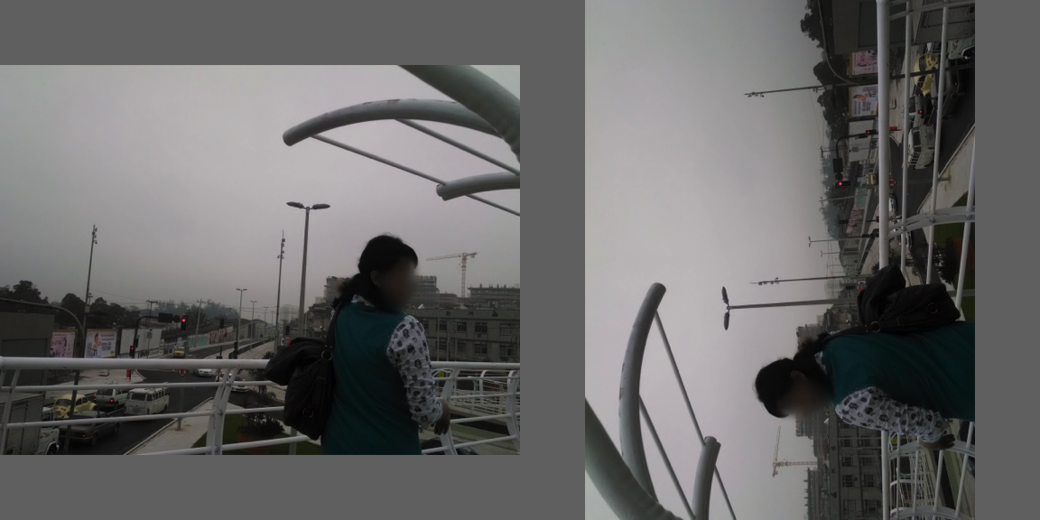
The dimensions are identical, because the canvas is square, and the model will still happily return boxes for the transposed image, just not the right ones.
transposed_x <- torch_tensor(aperm(transposed, c(3, 1, 2)), dtype = torch_float32())$div(255)$unsqueeze(1)
transposed_pred <- as.matrix(with_no_grad(model(transposed_x))$squeeze(1))
sum(transposed_pred[, 5] > CONF_THRESH)
# [1] 1
A square input cannot reveal this mistake through its dimensions. When in doubt, convert your array back into a raster and look at it.
Running the model on a single photograph
out <- with_no_grad(model(x))
out$shape
# [1]   1 300   6
The output is 1 × 300 × 6. YOLO26 always proposes 300 candidate boxes per image, and each one has six numbers. Let’s convert it to an R matrix and look at the first few rows.
pred <- as.matrix(out$squeeze(1))
colnames(pred) <- c("x1", "y1", "x2", "y2", "conf", "cls")
head(pred)
#             x1       y1       x2       y2      conf cls
# [1,] 222.09978 390.0912 229.8849 406.8148 0.8062587   9
# [2,] 152.45433 475.8222 209.2231 511.7309 0.7148697   5
# [3,] 394.51849 287.5258 556.1880 555.1393 0.7108306   0
# [4,] 105.64748 475.7938 161.2973 505.6293 0.6558898   2
# [5,]  61.18729 488.2326 148.1961 550.4704 0.5988283   2
# [6,] 324.12228 287.8313 556.1091 555.1833 0.4970481   0
x1, y1is the top-left corner of a box andx2, y2is its bottom-right corner, in the pixel coordinates of the padded 640 × 640 image, with y counting down from the top.confis the model’s confidence (0–1) that the box contains an object.clsis the index of the object class.
Most of the 300 candidates are junk. The confidence scores fall off quickly.
tibble(conf = pred[, "conf"]) %>%
  ggplot(aes(x = conf)) +
  geom_histogram(bins = 50) +
  geom_vline(xintercept = CONF_THRESH, linetype = "dashed") +
  labs(x = "confidence", y = "number of candidate boxes") +
  theme_minimal()
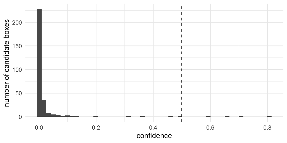
We keep only the candidates above a threshold. The threshold is a choice you make, not something the model tells you. Lower it and you find more objects, and more false ones.
keep <- pred[, "conf"] > CONF_THRESH
sum(keep)
# [1] 5
pred[keep, ]
#             x1       y1       x2       y2      conf cls
# [1,] 222.09978 390.0912 229.8849 406.8148 0.8062587   9
# [2,] 152.45433 475.8222 209.2231 511.7309 0.7148697   5
# [3,] 394.51849 287.5258 556.1880 555.1393 0.7108306   0
# [4,] 105.64748 475.7938 161.2973 505.6293 0.6558898   2
# [5,]  61.18729 488.2326 148.1961 550.4704 0.5988283   2
The class column contains numbers, not names. YOLO26 was trained on COCO, so the numbers identify COCO’s 80 categories. The Python ultralytics package would look these up for us. Here we need the lookup table ourselves. It is a small CSV file, coco_classes.csv, with one row per class. Download it into your InputData folder.
coco_classes <- here('InputData', 'coco_classes.csv') %>% read_csv
coco_classes
# # A tibble: 80 x 2
#    class_id class
#       <dbl> <chr>
#  1        0 person
#  2        1 bicycle
#  3        2 car
#  4        3 motorcycle
#  5        4 airplane
#  6        5 bus
#  7        6 train
#  8        7 truck
#  9        8 boat
# 10        9 traffic light
# # i 70 more rows
The class_id column uses the same numbering as the model, which starts at 0. Attaching names to the detections is then a join: each detection is matched to the row of coco_classes with the same class_id.
tibble(class_id = pred[keep, "cls"]) %>%
    left_join(coco_classes, by = "class_id", relationship = "many-to-one")
# # A tibble: 5 x 2
#   class_id class
#      <dbl> <chr>
# 1        9 traffic light
# 2        5 bus
# 3        0 person
# 4        2 car
# 5        2 car
A join matches rows by value, not by position, so there is no need to worry that R counts from 1 while the model counts from 0. left_join() keeps every detection, even one whose number is missing from the table (its class would be NA). relationship = "many-to-one" states what we expect: many detections can share a class, but each detection must match at most one row of the table. If the table ever contained a duplicated class_id, the join would stop with an error instead of quietly duplicating detections.
Mapping boxes back to the photograph
The boxes are in padded 640 × 640 coordinates. To place them on the original photograph, we undo the letterboxing in reverse order: subtract the padding, then divide by the scale.
boxes <- pred[keep, 1:4, drop = FALSE]
boxes[, c("x1", "x2")] <- (boxes[, c("x1", "x2")] - left) / scale
boxes[, c("y1", "y2")] <- (boxes[, c("y1", "y2")] - top)  / scale

detections <- tibble(
    file  = example_path,
    xmin  = boxes[, "x1"], ymin = boxes[, "y1"],
    xmax  = boxes[, "x2"], ymax = boxes[, "y2"],
    conf  = pred[keep, "conf"],
    class_id = pred[keep, "cls"]
) %>%
    left_join(coco_classes, by = "class_id", relationship = "many-to-one")
detections %>% select(-file) %>% arrange(desc(conf))
# # A tibble: 5 x 7
#    xmin  ymin  xmax  ymax  conf class_id class
#   <dbl> <dbl> <dbl> <dbl> <dbl>    <dbl> <chr>
# 1 1122. 1566. 1161. 1650. 0.806        9 traffic light
# 2  770. 1999. 1057. 2180. 0.715        5 bus
# 3 1992. 1048. 2809. 2399. 0.711        0 person
# 4  534. 1999.  815. 2149. 0.656        2 car
# 5  309. 2062.  748. 2376. 0.599        2 car
We now have 5 detections, each with a location in the original 3,232 × 2,424 photograph. Note that ymin is the top of each box, because these are still image coordinates.
Plotting the bounding boxes
To draw boxes on the photograph, we need to reconcile the two coordinate conventions from earlier. plotRGB() draws the raster in map coordinates, with y = 0 at the bottom, so each box’s image y coordinates have to be flipped against the photograph’s height: h - ymax becomes the bottom of the box and h - ymin becomes the top. Base R’s rect() and text() then draw on top of the raster in those same coordinates.
class_colors <- c(car = "#E4572E", person = "#17BEBB", bus = "#FFC914",
                  truck = "#76B041", motorcycle = "#A05195", bicycle = "#2E86AB")

plot_detections <- function(path, dets, classes_of_interest = names(class_colors)) {
    r <- rast(path)
    h <- nrow(r)
    d <- dets %>% filter(class %in% classes_of_interest)

    plotRGB(r, mar = c(0, 0, 0, 0))
    if (nrow(d) == 0) return(invisible())   # text() fails on zero labels
    rect(d$xmin, h - d$ymax, d$xmax, h - d$ymin,
         border = class_colors[d$class], lwd = 2)
    text(d$xmin, h - d$ymin, sprintf("%s %.2f", d$class, d$conf),
         col = "white", cex = 0.7, adj = c(0, -0.3))
}
plot_detections(example_path, detections)
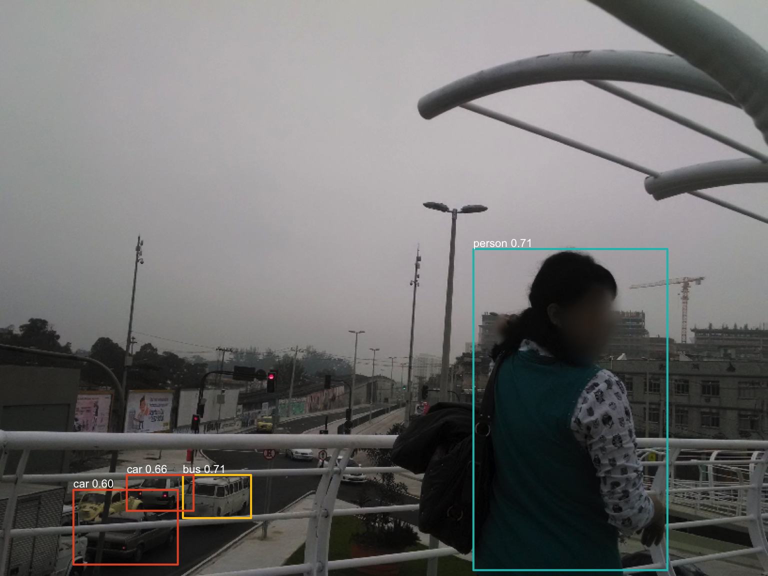
Try removing the h - from the rect() call. The boxes will still be drawn, with the right sizes, in the wrong places: mirrored top to bottom.
Two things worth knowing if you adapt this for your own model:
jit_load()’d TorchScript modules don’t reliably supportmodel$eval()/model$train(FALSE)as oftorch0.17.0 +libtorch2.8.0; it fails with an internal S3-dispatch error on scripted modules. This particular export is safe to skip that call on: Ultralytics’ export log reports the model already “fused” (BatchNorm folded into the convolution weights), and a side-by-side Python comparison calling vs. skippingmodel.eval()on the same file gives bit-identical output. If you export a custom or non-fused model, re-check this.- On Ultralytics’ own
bus.jpgsample image, this pipeline and the Pythonultralyticspackage (running the same TorchScript file) agree closely: 0.97 vs 0.97 confidence on the bus, and 0.94/0.94/0.91/0.71 vs 0.94/0.94/0.91/0.63 on the four people in frame. The two paths decode and resample the image with different libraries (GDAL here, OpenCV in Python), so don’t expect bit-identical confidences.
Cropping detections out of the raster
A bounding box is a rectangular extent, and cropping a raster to an extent is one of the most common raster operations. Here we use terra::crop(). As with plotting, the image y coordinates must be flipped into the raster’s map y coordinates.
crop_detection <- function(r, det) {
    h <- nrow(r)
    crop(r, ext(det$xmin, det$xmax, h - det$ymax, h - det$ymin))
}

vehicles <- detections %>% filter(class %in% c("car", "bus", "truck"))
vehicle_crops <- map(seq_len(nrow(vehicles)), ~ crop_detection(example_rast, vehicles[.x, ]))
par(mfrow = c(1, length(vehicle_crops)), mar = c(0, 0, 1, 0))
walk2(vehicle_crops, vehicles$class, ~ plotRGB(.x, main = .y))
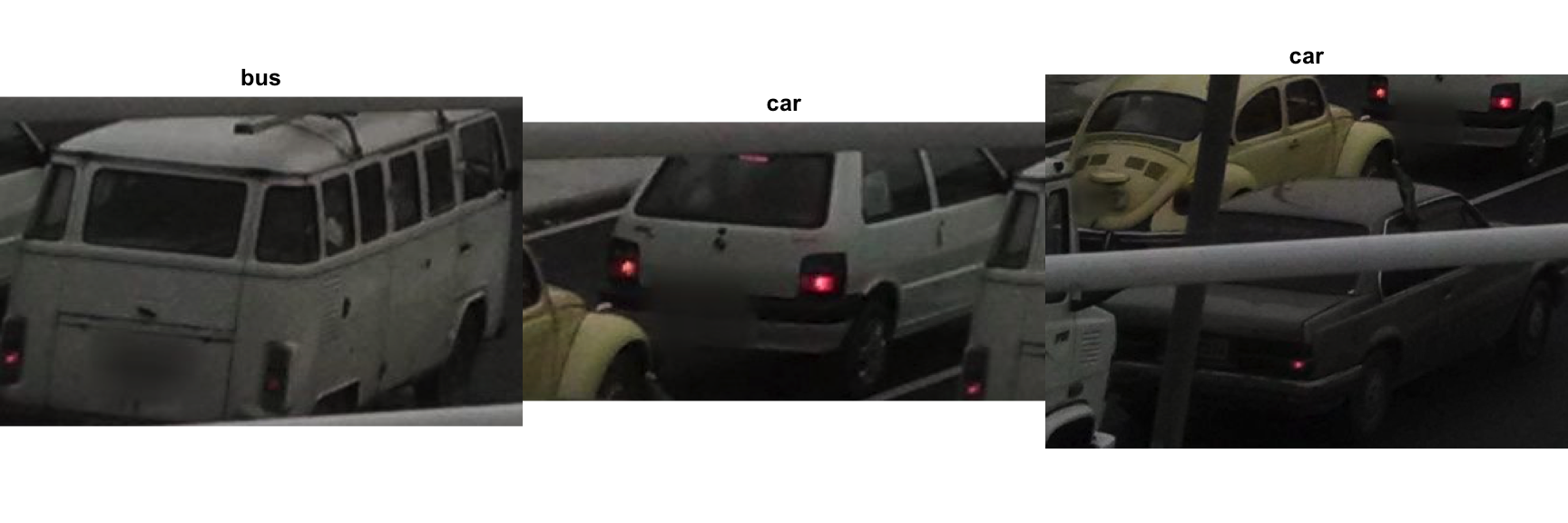
Each crop is itself a raster, so anything you can do with a raster, you can do with a detected object. For example, the mean colour of each vehicle, and the share of the photograph each one takes up:
vehicles %>%
    mutate(
        mean_red   = map_dbl(vehicle_crops, ~ global(.x$red,   "mean")$mean),
        mean_green = map_dbl(vehicle_crops, ~ global(.x$green, "mean")$mean),
        mean_blue  = map_dbl(vehicle_crops, ~ global(.x$blue,  "mean")$mean),
        share_of_image = (xmax - xmin) * (ymax - ymin) / (w * h)
    ) %>%
    select(class, conf, starts_with("mean"), share_of_image)
# # A tibble: 3 x 6
#   class  conf mean_red mean_green mean_blue share_of_image
#   <chr> <dbl>    <dbl>      <dbl>     <dbl>          <dbl>
# 1 bus   0.715     72.6       71.8      68.2        0.00664
# 2 car   0.656     62.1       60.4      55.8        0.00540
# 3 car   0.599     50.6       49.0      45.0        0.0176
The share of the image is a crude proxy for distance. Nearby vehicles take up more of the frame than distant ones. It is crude because a bus far away and a car close by can take up the same area.
Exercise
- The object labelled
busis a Volkswagen Kombi van. Is that label right? What does it tell you about how COCO’s categories map onto the vehicles you care about? - The larger
carcrop also contains most of a yellow Beetle and the bridge railing. Why is the mean a poor summary of an object’s colour? What else is inside the box? - Crop the person detection instead. How many pixels tall is the person in the original photograph? What would it be in the 640 × 640 image the model saw?
- Lower
CONF_THRESHto 0.25 and re-run this section. What shows up that wasn’t there before, and would you trust it?
Turning the steps into functions
So far, every step has been written for one photograph. To run it on hundreds, we collect the steps into functions. They are a direct copy of the code above, with one change, explained in the next section.
letterbox <- function(path, size = IMG_SIZE) {
    r <- rast(path)
    w <- ncol(r); h <- nrow(r)
    ext(r) <- ext(0, w, 0, h)

    scale <- min(size / w, size / h)   # longer side becomes `size`
    new_w <- round(w * scale); new_h <- round(h * scale)
    template <- rast(nrows = new_h, ncols = new_w, nlyrs = 3, extent = ext(r), crs = crs(r))
    resized <- resample(r, template, method = "average")

    left <- (size - new_w) %/% 2L; top <- (size - new_h) %/% 2L
    ext(resized) <- ext(left, left + new_w, size - top - new_h, size - top)
    padded <- extend(resized, ext(0, size, 0, size), fill = PAD_VALUE)

    list(raster = padded, scale = scale, left = left, top = top, orig_w = w, orig_h = h)
}

raster_to_tensor <- function(r) {
    arr <- as.array(r)   # height, width, channel
    torch_tensor(aperm(arr, c(3, 1, 2)), dtype = torch_float32())$div(255)$unsqueeze(1)
}

detect_image <- function(path, conf_thresh = CONF_THRESH) {
    lb <- letterbox(path)
    pred <- as.matrix(with_no_grad(model(raster_to_tensor(lb$raster)))$squeeze(1))

    keep  <- pred[, 5] > conf_thresh
    boxes <- pred[keep, 1:4, drop = FALSE]
    boxes[, c(1, 3)] <- (boxes[, c(1, 3)] - lb$left) / lb$scale
    boxes[, c(2, 4)] <- (boxes[, c(2, 4)] - lb$top)  / lb$scale

    tibble(
        file  = path,
        xmin  = boxes[, 1], ymin = boxes[, 2],
        xmax  = boxes[, 3], ymax = boxes[, 4],
        conf  = pred[keep, 5],
        class_id = pred[keep, 6]
    ) %>%
        left_join(coco_classes, by = "class_id", relationship = "many-to-one")
}
Always check a new function against a result you already know. It should reproduce the detections from the previous sections exactly.
all.equal(detect_image(example_path), detections)
# [1] TRUE
A photograph that does not fit
When we worked through the example photograph, we scaled it by its width, because the width was the longer side. That was a fact about one photograph, not about the data. As the table of image sizes showed, some photographs are in portrait orientation. letterbox() therefore scales by whichever side is longer, which is the same as taking the smaller of the two scale factors: min(size / w, size / h). A landscape photograph is padded at the top and bottom, and a portrait one on the left and right.
portrait_path <- img_files_paths[str_detect(img_files_paths, "204024303")]
portrait_dets <- detect_image(portrait_path)

par(mfrow = c(1, 2))
plotRGB(letterbox(portrait_path)$raster)   # what the model sees
plot_detections(portrait_path, portrait_dets)
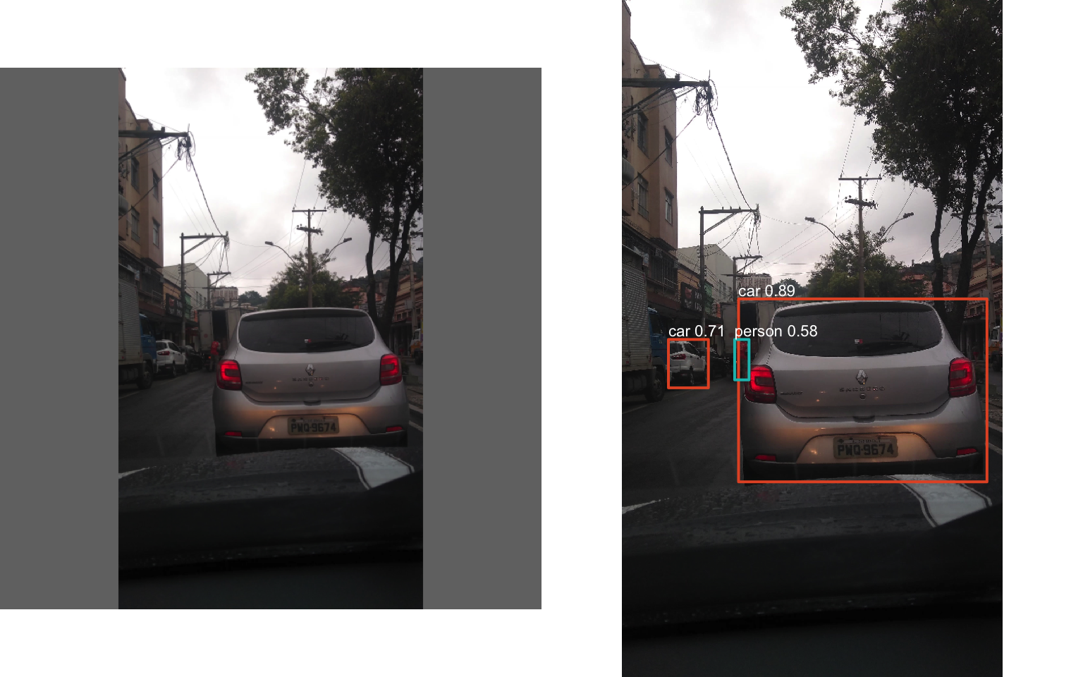
A pipeline built and tested on one example contains that example’s assumptions, whether you wrote them down or not. Test it on the data that differs most from your example before you trust it on the rest.
A photograph with nothing in it
Some photographs genuinely contain nothing the model recognises.
empty_path <- img_files_paths[str_detect(img_files_paths, "1319868701")]
detect_image(empty_path)
# # A tibble: 0 x 8
# # i 8 variables: file <chr>, xmin <dbl>, ymin <dbl>, xmax <dbl>, ymax <dbl>,
# #   conf <dbl>, class_id <dbl>, class <chr>
plotRGB(rast(empty_path))
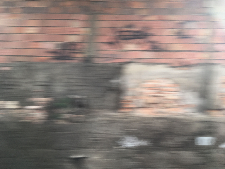
This is a motion-blurred wall. detect_image() returns a tibble with the right columns and zero rows, which is what we want. “Zero detections” is a legitimate output. But zero-row results have a way of disappearing when results are combined across images, as we’ll see next.
Exercise
- Change
scale <- min(size / w, size / h)inletterbox()back toscale <- size / w, the assumption we made for the example photograph, and rundetect_image(portrait_path)insidetry(). Read the error message. Does it tell you what is wrong with your code? - When a model complains about its input, check the input. With the width-only scale, what is
dim(letterbox(portrait_path)$raster)? Work outnew_handtopby hand for this 2,340 × 4,160 photograph. Why doesn’textend()produce a 640 × 640 raster? - Suppose
letterbox()had forced the result to 640 × 640 by cropping it, withcrop(padded, ext(0, size, 0, size)). Plot the result. Which parts of the photograph does the model no longer see? Compare the detections with those from the correctletterbox(). Why is a pipeline that quietly runs on a cropped image more dangerous than one that stops with an error? - Instead of letterboxing, stretch the portrait photograph to 640 × 640 by resampling it to a 640 × 640 template and run the model on it. Are the detections better or worse? How would you have to change the box mapping to handle a stretched image?
- Change the resampling
methodinletterbox()to"near"and then"bilinear", and rerun the example photograph. Do the detections change? Plot a zoomed-in crop of each resampled raster to see why. - Find the images that are neither 3,072 × 1,728 nor portrait in
img_metadata. Check that the letterboxed version of one of them looks right.
Defensive programming and scaling up
The portrait photograph showed how far an error can surface from its cause. The mistake was in letterbox(), but the error came from inside the model and was reported as a problem with as.matrix(). Defensive programming means checking your assumptions at the point where your code depends on them, and stopping with a message that names the actual problem.
Our pipeline makes several assumptions without saying so:
- The file exists.
- The image has exactly three bands: red, green and blue.
- Pixel values run from 0 to 255 (8 bits per band), so that dividing by 255 puts them between 0 and 1.
- The letterboxed raster is exactly 640 × 640 × 3.
- The model returns 300 candidate boxes with 6 numbers each.
To see why these matter, let’s make two images that break them. A greyscale image has one band. Many scientific and drone images store 16 bits per band, with values from 0 to 65,535. We create both from the example photograph and save them to temporary files.
grey_path <- file.path(tempdir(), "greyscale.tif")
writeRaster(mean(example_rast), grey_path, overwrite = TRUE)   # 1 band

deep_path <- file.path(tempdir(), "16bit.tif")
writeRaster(example_rast * 256, deep_path, datatype = "INT2U", overwrite = TRUE)   # 16-bit values
The greyscale image fails with the same unhelpful message as the portrait photograph.
attempt <- try(detect_image(grey_path), silent = TRUE)
conditionMessage(attr(attempt, "condition")) %>% str_extract("^[^\n]*")
# [1] "error in evaluating the argument 'x' in selecting a method for function 'as.matrix': The following operation failed in the TorchScript interpreter."
The 16-bit image is worse. It does not fail at all.
detect_image(deep_path)
# # A tibble: 0 x 8
# # i 8 variables: file <chr>, xmin <dbl>, ymin <dbl>, xmax <dbl>, ymax <dbl>,
# #   conf <dbl>, class_id <dbl>, class <chr>
Its pixel values, divided by 255, run up to about 256 instead of 1. The model sees garbage and finds nothing. Without an error, this photograph would silently count as having zero cars.
Checking assumptions
We write two small functions that check assumptions 1–4, and call stop() with a clear message when one fails. call. = FALSE leaves out the function call from the message, which makes it easier to read.
check_image <- function(path) {
    if (!file.exists(path)) {
        stop("file not found: ", path, call. = FALSE)
    }
    r <- rast(path)
    if (nlyr(r) != 3) {
        stop(basename(path), " has ", nlyr(r), " band(s); expected 3 (red, green, blue)", call. = FALSE)
    }
    invisible(r)
}

check_letterbox <- function(lb, size = IMG_SIZE) {
    d <- dim(lb$raster)
    if (!identical(as.numeric(d), c(size, size, 3))) {
        stop("letterboxed raster is ", paste(d, collapse = " x "),
             "; the model needs ", size, " x ", size, " x 3", call. = FALSE)
    }
    v <- range(values(lb$raster))
    if (anyNA(v)) {
        stop("letterboxed raster contains missing values", call. = FALSE)
    }
    if (v[1] < 0 || v[2] > 255) {
        stop("pixel values run from ", round(v[1]), " to ", round(v[2]),
             "; expected 0 to 255 (8 bits per band)", call. = FALSE)
    }
    invisible(lb)
}
The value check runs on the small letterboxed raster rather than on the full photograph. It adds a few milliseconds per image, which is negligible next to the model itself.
Now detect_image() calls the checks before the model does anything. It also checks the shape of the model’s output, using stopifnot(). stopifnot() stops if any of its conditions is FALSE, and the name of each condition becomes the error message.
detect_image <- function(path, conf_thresh = CONF_THRESH) {
    check_image(path)
    lb <- check_letterbox(letterbox(path))
    pred <- as.matrix(with_no_grad(model(raster_to_tensor(lb$raster)))$squeeze(1))
    stopifnot("model output is not 300 x 6" = identical(dim(pred), c(300L, 6L)))

    keep  <- pred[, 5] > conf_thresh
    boxes <- pred[keep, 1:4, drop = FALSE]
    boxes[, c(1, 3)] <- (boxes[, c(1, 3)] - lb$left) / lb$scale
    boxes[, c(2, 4)] <- (boxes[, c(2, 4)] - lb$top)  / lb$scale

    tibble(
        file  = path,
        xmin  = boxes[, 1], ymin = boxes[, 2],
        xmax  = boxes[, 3], ymax = boxes[, 4],
        conf  = pred[keep, 5],
        class_id = pred[keep, 6]
    ) %>%
        left_join(coco_classes, by = "class_id", relationship = "many-to-one")
}

all.equal(detect_image(example_path), detections)   # good images are unaffected
# [1] TRUE
Each bad input now fails at the point where the assumption is broken, with a message that says what is wrong.
try(detect_image("no_such_file.jpg"))
# Error : file not found: no_such_file.jpg
try(detect_image(grey_path))
# Error : greyscale.tif has 1 band(s); expected 3 (red, green, blue)
try(detect_image(deep_path))
# Error : pixel values run from 0 to 60809; expected 0 to 255 (8 bits per band)
Keeping a batch running
Stopping is the right response for a single photograph. It is the wrong response for a batch of 484, where one bad file would stop the whole run. purrr::safely() wraps a function so that it never stops. Instead, it returns a list with two elements, result and error, one of which is always NULL.
test_files <- c(example_path, portrait_path, grey_path, deep_path, "no_such_file.jpg")
results <- map(test_files, safely(detect_image))

tibble(
    file  = basename(test_files),
    error = map_chr(results, ~ if (is.null(.x$error)) "" else conditionMessage(.x$error))
) %>%
    knitr::kable()
| file | error |
|---|---|
| 1318411189__3645401_74b21_60c0ec1f7c728.jpg | |
| 204024303__1129811_162e7_50.jpg | |
| greyscale.tif | greyscale.tif has 1 band(s); expected 3 (red, green, blue) |
| 16bit.tif | pixel values run from 0 to 60809; expected 0 to 255 (8 bits per band) |
| no_such_file.jpg | file not found: no_such_file.jpg |
The good images give their detections, and every failure is recorded along with its reason.
map_dfr(results, "result") %>% count(file = basename(file), class)
# # A tibble: 6 x 3
#   file                                        class             n
#   <chr>                                       <chr>         <int>
# 1 1318411189__3645401_74b21_60c0ec1f7c728.jpg bus               1
# 2 1318411189__3645401_74b21_60c0ec1f7c728.jpg car               2
# 3 1318411189__3645401_74b21_60c0ec1f7c728.jpg person            1
# 4 1318411189__3645401_74b21_60c0ec1f7c728.jpg traffic light     1
# 5 204024303__1129811_162e7_50.jpg             car               2
# 6 204024303__1129811_162e7_50.jpg             person            1
This is different from wrapping code in try() to make errors go away. A failure is not discarded: it is kept in a table where you can count it, report it, and fix it. A batch that finishes with some failures is useful. A batch that finishes with no failures because they were silently dropped is not.
Running every photograph
With the checks in place, we can run all 484 photographs. This takes a couple of minutes.
results_all <- map(img_files_paths, safely(detect_image))

failures <- tibble(
    file  = basename(img_files_paths),
    error = map_chr(results_all, ~ if (is.null(.x$error)) NA_character_ else conditionMessage(.x$error))
) %>%
    filter(!is.na(error))

detections_all <- map_dfr(results_all, "result")
nrow(failures)
# [1] 0
nrow(detections_all)
# [1] 1980
detections_all %>% count(class, sort = TRUE)
# # A tibble: 15 x 2
#    class             n
#    <chr>         <int>
#  1 car            1457
#  2 person          206
#  3 bus             121
#  4 traffic light    87
#  5 truck            71
#  6 motorcycle       11
#  7 bicycle           9
#  8 umbrella          8
#  9 backpack          2
# 10 bench             2
# 11 fire hydrant      2
# 12 dog               1
# 13 handbag           1
# 14 potted plant      1
# 15 train             1
0 of the 484 photographs failed the checks. That is worth reporting: it says that every photograph was checked and passed, not that failures went unrecorded. The model found 1,980 objects. car dominates, as it did in the earlier post’s Rio sample, which is unsurprising for imagery collected from a car. The rare classes at the bottom of the table (umbrellas, a dog, a train) are worth looking at individually. Some will be right and some will be misclassifications.
Counting per photograph
Suppose we want the number of cars in each photograph. The obvious approach is to count the rows of detections_all by file.
cars_naive <- detections_all %>%
    filter(class == "car") %>%
    count(file, name = "car")

nrow(cars_naive)
# [1] 390
mean(cars_naive$car)
# [1] 3.735897
That table has only 390 rows, not 484. Photographs with no cars (like the wall above) produced no car rows in detections_all, so they cannot appear in a count of its rows. The mean is the average over photographs that have at least one car, which is not the same as the average over all photographs.
To keep them, we have to say which photographs and which classes should be there, and fill in the missing combinations with zero. complete() does exactly this.
counts <- detections_all %>%
    filter(class %in% c("car", "person", "bus")) %>%
    count(file, class) %>%
    complete(file = img_files_paths, class = c("car", "person", "bus"), fill = list(n = 0L)) %>%
    pivot_wider(names_from = class, values_from = n)

nrow(counts)
# [1] 484
mean(counts$car)
# [1] 3.010331
Now there is one row per photograph, and the average number of cars per photograph is 3.01 rather than 3.74.
Checking by eye
Summary tables and maps hide the individual mistakes. Before trusting the numbers, look at a random sample of photographs with their detections.
set.seed(42)
check_files <- sample(img_files_paths, 6)

par(mfrow = c(2, 3))
walk(check_files, function(p) {
    plot_detections(p, detections_all %>% filter(file == p))
})
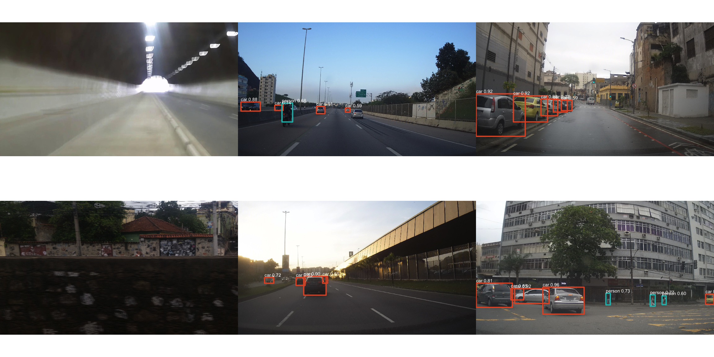
Note the empty panels (a tunnel, a wall glimpsed mid-motion) where nothing cleared the confidence threshold, the doubled-up labels where two boxes overlap closely enough that their text collides, and the motorcyclist who is detected as a person but whose motorcycle is not. This is the kind of real-world messiness that a single cherry-picked example photo hides.
Exercise
- Replace
scale <- min(size / w, size / h)inletterbox()withscale <- size / wagain, and run the newdetect_image()onportrait_path. Compare the error message with the one you got earlier. - Should a 16-bit image be rejected, or converted? Write a version of
check_letterbox()that rescales 16-bit values to 0–255 instead of stopping. What would you need to know about the image to do this safely? - After the boxes are mapped back to the original photograph, add a check that they lie inside it (between 0 and the photograph’s width and height). Run it over all the photographs. Do any boxes fall outside? What should the function do when they do?
- Put the counts on a map.
img_metadataalready holds the GPS coordinates of every photograph. Join it tocountsby file name (img_metadatauses the columnFileName, which isbasename(file)), and userelationship = "one-to-one"so the join checks that each photograph matches exactly one row. PlotGPSLongitudeagainstGPSLatitude, coloured by the number of cars, withcoord_quickmap(). What does the map show, and what does it not show? Think about the direction the camera was facing, the lighting, the time of day, and whether the car carrying the camera was stuck in traffic. - Repeat the map for
persondetections. Where are pedestrians most and least visible? - Find the photographs with the rare classes (
umbrella,dog,trainand so on) and plot their detections. How many are correct? - The
classes_of_interestfilter inplot_detections()silently drops everything else the model found. Remove the filter for one image. What else is in a typical street scene that a transportation-focused analysis would otherwise never see? - Compare this model’s detections on the same photograph against the YOLOv10 results from the earlier post. Do the two models agree on classes and confidences? Where do they diverge?
Conclusion
Dropping reticulate and a Python environment out of the pipeline trades one kind of complexity for another. There’s no conda environment to set up and no use_condaenv() path to get right for Windows versus Mac. In exchange, R takes on the work that ultralytics$YOLO() used to do invisibly: resampling, padding, array layout, box coordinates, even the COCO class names. Each of those is a raster operation, and most of them can go wrong without an error: the wrong cell order transposes the photograph, a scale factor chosen for landscape photographs breaks on portrait ones, and a count that starts from the detections forgets the photographs with none. In every case the remedy was the same: look at the raster the model actually received, and test the code on data that doesn’t match the example it was written for.
The caveats from the earlier post apply just as much here. This is still a pre-trained model applied with no fine-tuning, still liable to misclassify, still liable to miss things in fog, poor lighting, or partial occlusion, still trained on a dataset (COCO) whose composition shapes what it notices and what it doesn’t. Whether the inference happens in Python or in R has no bearing on any of that. Treat what comes out of either pipeline as a starting point for human review, not a finished count.
Nikhil Kaza
Professor
My research interests include urbanization patterns, local energy policy and equity