Analysing Urban Neworks
Introduction
Networks are ubiquitous in a urban systems. The more obvious ones are street, rail and utility networks that undergird the city. However, as planners we also focus on less obvious networks; e.g. social networks of people that allow for community formation, the transactional activity of firms that allow us to identify clusters of firms or industries, the mismatch between job seekers and job locations to better plan for social and physical infrastructure and information flow through organisational linkages during a disaster management process. These are but a few examples of network analysis in the urban domain. The problem definition frames the analytical tools used in the process.
Acquire Data
Let’s begin by using the bike share data from New York, we are familiar with. We already did some network analysis with it (inadvertently). Let’s formalise it. Much of the following data cleaning that you should be familiar with now.
Key nodes in a network
Networks are representation of connections between two nodes. As such bike stations, could be treated a vertex/node and each trip between any two stations could be treated as a link. In another representation, you can treat all stations connected with one another, if they belong to the same company that you can check out and return these bikes and treat the number of trips as weights on that edge; so some edges will have zero weights. In other instances, you may disallow edges that have zero weights, i.e. remove the connection between two stations if there are no trips between them (or number of trips below a threshold).
library(tidyverse)
library(igraph)
library(here)


tripdata <- here("tutorials_datasets", "nycbikeshare", "201806-citibike-tripdata.csv") %>% read_csv()

tripdata <- rename(tripdata,              #rename column names to get rid of the space
                   Slat = `start station latitude`,
                   Slon = `start station longitude`,
                   Elat = `end station latitude`,
                   Elon = `end station longitude`,
                   Sstid = `start station id`,
                   Estid = `end station id`,
                   Estname = `end station name`,
                   Sstname = `start station name`

)
diffdesttrips <- tripdata[tripdata$Estid != tripdata$Sstid, ] # to make sure there are no loops or self-connections.


(trips_graph <- diffdesttrips %>%
        select(Sstid,Estid) %>%
        graph.data.frame(directed = T)) #We are using directed graph because the links have from and to edges. You can choose to ignore them.
# IGRAPH 2b31606 DN-- 773 1909858 --
# + attr: name (v/c)
# + edges from 2b31606 (vertex names):
#  [1] 72->173  72->477  72->457  72->379  72->459  72->446  72->212  72->458
#  [9] 72->212  72->514  72->514  72->465  72->173  72->524  72->173  72->212
# [17] 72->382  72->462  72->3141 72->456  72->519  72->328  72->426  72->3659
# [25] 72->359  72->525  72->405  72->458  72->457  72->3163 72->426  72->328
# [33] 72->376  72->3459 72->304  72->457  72->486  72->527  72->490  72->459
# [41] 72->459  72->3178 72->3178 72->515  72->459  72->388  72->500  72->508
# [49] 72->173  72->426  72->368  72->3258 72->532  72->478  72->514  72->533
# [57] 72->519  72->423  72->3457 72->525  72->525  72->490  72->529  72->405
# + ... omitted several edges


vcount(trips_graph)
# [1] 773
ecount(trips_graph)
# [1] 1909858
is.directed(trips_graph)
# [1] TRUE
You can access the vertices and edges using V and E functions.
V(trips_graph) %>% head()
# + 6/773 vertices, named, from 2b31606:
# [1] 72  79  82  83  119 120
E(trips_graph) %>% head()
# + 6/1909858 edges from 2b31606 (vertex names):
# [1] 72->173 72->477 72->457 72->379 72->459 72->446

tmp1 <- diffdesttrips %>%
  group_by(Sstid) %>%
  summarise(
    stname = first(Sstname),
    lon = first(Slon),
    lat = first(Slat))%>%
  rename(stid = Sstid)

tmp2 <- diffdesttrips %>%
  group_by(Estid) %>%
  summarise(
    stname = first(Estname),
    lon = first(Elon),
    lat = first(Elat)) %>%
  rename(stid = Estid)

station_locs <- rbind(tmp1, tmp2) %>% unique()
You can extract subgraphs for a subset of vertices
set.seed(200) # For reproducibility because of randomisation below
station_sample <- sample(V(trips_graph), 20)
sub_trips <- induced_subgraph(trips_graph, station_sample)


# plot using ggraph
library(ggraph)
ggraph(sub_trips, layout = 'kk') +
    geom_edge_fan(show.legend = FALSE) +
    geom_node_point()
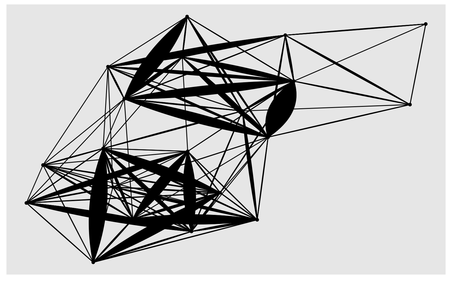
Note that the graph does not respect the geographic locations. If you want to fix the positions relative to their lat/long coordinates, you should can specify them using layout parameters.
Exercise
- Use different layouts (such as star and cricle) to visualise the network.
- Use different edge attributes to style the edges of the above graph
- Style the vertices using for e.g. number of incoming trips per day, or their location in different boroughs.
Adjacency matrix
One representation of a graph is an adjacency matrix. It is a square matrix used to represent a finite graph. The elements of the matrix indicate whether pairs of vertices are adjacent or not in the graph. Each row and each column represents a single vertex. $ A $ is and adjacency matrix, whose elements $ a_{ij} $ is 0 when vertices/nodes $ i $ and $ j $ are not adjacent. If the graph is undirected and unweighted then $ a_{ij} $ is 1 when they are adjacent. In the case of a directed graph, the matrix is not symmetric. In our case, we have a weighted directed graph with the weights representing the number of trips between two stations. To visualise a portion of this matrix try
as_adjacency_matrix(trips_graph)[1:6, 1:6]
# 6 x 6 sparse Matrix of class "dgCMatrix"
#     72 79 82 83 119 120
# 72   .  7  .  .   .   .
# 79  22  .  3  .   1   .
# 82   1  3  .  .   .   .
# 83   .  .  .  .   2  18
# 119  .  .  1  1   .   1
# 120  .  .  . 20   .   .
Adjacency matrix is very important as it allows us to perform matrix operations much more efficiently as we will see in other tutorials
Degrees & their distribution.
Degree of a vertex, in graph theory, refers to the number of edges that has the vertex as one of its ends. An in-degree and out-degree qualifies it, by counting only edges that start and end at the vertex. Degree distributions are important for graphs as they tell us about how connected the graph is and which if any of the vertices are more important than others.
degree(trips_graph, mode = 'out') %>%
  as.tibble %>%
  ggplot()+
  geom_density(aes(x=value))
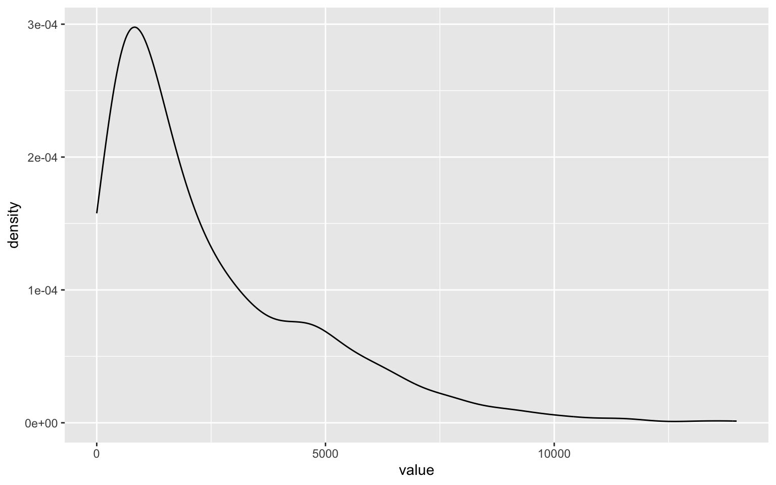
degree.distribution(trips_graph) %>% head() # Check out what the degree.distribution produces and how to interpret the results.
# [1] 0.000000000 0.003880983 0.005174644 0.002587322 0.001293661 0.001293661
In particular, you want to look for the outliers in the distribution. For example to find the stations with only end trips but no start trips, i.e stations that are solely destinations
V(trips_graph)$name[degree(trips_graph, mode="out") == 0 & degree(trips_graph, mode="in") > 0]
#  [1] "3245" "3267" "3275" "3192" "3276" "3184" "3214" "3651" "3198" "3199"
# [11] "3203"
We can also visualise these stations that are popular origins on the map. However, we need to attach the values to the station locations tibble.
tmp <- degree(trips_graph, mode = 'out') %>%
  as.tibble() %>%
  rename(Outdegree = value)%>%
  mutate(stid = V(trips_graph)$name %>% as.numeric())


station_locs <- station_locs %>%
  left_join(tmp, by='stid')


library(tmap)
library(sf)

tmap_mode("view")

m1 <-
station_locs %>%
  mutate(outdegree_std = (Outdegree - mean(Outdegree))/sd(Outdegree)) %>%
  filter(outdegree_std >2) %>% # focusing on the Outliers!
  st_as_sf(coords = c('lon', 'lat'), crs=4326) %>%
  tm_shape()+
  tm_dots(size = 'outdegree_std', alpha =.5, border.lwd=0)+
  tm_basemap(leaflet::providers$CartoDB)


# Showing the use of leaflet  and fillcolorfor reference

# library(leaflet)
#
#  Npal <- colorNumeric(
#    palette = "Reds", n = 5,
#    domain = station_locs$Outdegree
#  )
#
#  m1 <-
# station_locs %>%
#     leaflet()  %>%
#   addProviderTiles(providers$CartoDB.Positron, group = "Basemap") %>%
#    addCircles(
#      lng = station_locs$lon,
#      lat = station_locs$lat,
#      radius = (station_locs$Outdegree - mean(station_locs$Outdegree))/sd(station_locs$Outdegree) * 30,
#      fillOpacity = .6,
#     fillColor = Npal(station_locs$Outdegree),
#      group = 'Stations',
#      stroke=FALSE
#    ) %>%
#   addLegend("topleft", pal = Npal, values = ~Outdegree,
#             labFormat = function(type, cuts, p) {
#               n = length(cuts)
#               paste0(prettyNum(cuts[-n], digits=2, big.mark = ",", scientific=F), " - ", prettyNum(cuts[-1], digits=2, big.mark=",", scientific=F))
#             },
#             title = "Out degree/Trip Starts",
#             opacity = 1
#   )

library(widgetframe)
frameWidget(tmap_leaflet(m1))
You can also find out which stations are predominantly origin stations and which are predominantly destinations. I use 20% more as a cut off (arbitrary).
# Careful with division. If you have a nodes that are only origins, i.e. in-degree is 0, you will have a division by 0 problem.

V(trips_graph)$name[degree(trips_graph, mode="out") / degree(trips_graph, mode="in") > 1.2]
#  [1] "216"  "258"  "266"  "289"  "339"  "356"  "391"  "397"  "399"  "443"
# [11] "469"  "3152" "3161" "3164" "3177" "3302" "3316" "3366" "3536" "3539"
# [21] "3542" "3620" "3623"
Exercise
- Identify the popular origin stations of the trips by different times of the day and day of the week
- Modify the above code slightly to identify the popular destinations by different times of the day and day of the week.
Other centrality measures
Eigen centrality
If $ A = a_{ij} $ be the adjacency matrix of a graph, where $ a_{ij} = 1 $ when $ i $ and $ j $ nodes are connected, $ 0 $ otherwise. The eigenvector centrality $ x_{i} $ of node $ i $ is given by:
$$ x_i = \frac{1}{\lambda} \sum_{k} a_{ki} x_k $$
where $ $ is a constant and is the largest eigen value of the adjacency matrix.
Intuitively, a node is considered more central/important, if it is connected to large number of highly central/important nodes. So, a node may have a high degree score (i.e. many connections) but a relatively low eigen centrality score if many of those connections are with similarly low-scored nodes.
station_locs$eigencentrality <- eigen_centrality(trips_graph, directed = T)$vector
Showing only the stations with large eigen centrality scores.
Page rank centrality
Page rank is a version of eigen centrality, made popular by the founders of Google. We can use boxplot in the standard graphics package to identify the outliers. .
tmp  <- page_rank(trips_graph)$vector %>%
    boxplot.stats() %>%
    .[["out"]] %>% ## Box plot identifies the oultiers, outside the whiskers. The default value is 1.5 outside the box.
     names() %>%
    as.numeric()

station_locs %>%
  filter(stid %in% tmp) %>%
  select('stname')
# # A tibble: 17 × 1
#    stname
#    <chr>
#  1 Broadway & E 14 St
#  2 Christopher St & Greenwich St
#  3 Carmine St & 6 Ave
#  4 Centre St & Chambers St
#  5 Broadway & E 22 St
#  6 West St & Chambers St
#  7 W 21 St & 6 Ave
#  8 W 41 St & 8 Ave
#  9 8 Ave & W 33 St
# 10 W 33 St & 7 Ave
# 11 E 17 St & Broadway
# 12 Broadway & W 60 St
# 13 12 Ave & W 40 St
# 14 Pershing Square North
# 15 Central Park S & 6 Ave
# 16 South End Ave & Liberty St
# 17 Kent Ave & N 7 St
Closeness centrality
While the above measures of centrality depend on local neighbourhood, we can also take into account the whole graph. For example, if a station can every station within a few hops, then it is considered more central than ones that may have more localised trips within the neighbourhood.
tmp <- closeness(trips_graph, mode='all') %>%
  boxplot.stats() %>%
  .[['out']] %>%
   names() %>%
    as.numeric()

station_locs %>%
  filter(stid %in% tmp) %>%
  select('stname')
# # A tibble: 7 × 1
#   stname
#   <chr>
# 1 Paulus Hook
# 2 Liberty Light Rail
# 3 Heights Elevator
# 4 Hamilton Park
# 5 Essex Light Rail
# 6 Morris Canal
# 7 Bike Mechanics at Riis
These seems like unusual stations to be outliers in a centrality index (bike mechanics??) and unlike the page rank index. A closer look at the centrality using box plot reveals that these are outliers at the left end of the centrality distribution.
There are hundreds of centrality measures out there. Be careful to pick and choose the right ones for your problem. To assist with this, you can use CINNA (Central Informative Nodes in Network Analysis) package for computing, analysing and comparing centrality measures submitted to CRAN repository.
library(CINNA)
proper_centralities(trips_graph)
#  [1] "Alpha Centrality"
#  [2] "Bonacich power centralities of positions"
#  [3] "Page Rank"
#  [4] "Average Distance"
#  [5] "Barycenter Centrality"
#  [6] "BottleNeck Centrality"
#  [7] "Centroid value"
#  [8] "Closeness Centrality (Freeman)"
#  [9] "ClusterRank"
# [10] "Decay Centrality"
# [11] "Degree Centrality"
# [12] "Diffusion Degree"
# [13] "DMNC - Density of Maximum Neighborhood Component"
# [14] "Eccentricity Centrality"
# [15] "Harary Centrality"
# [16] "eigenvector centralities"
# [17] "K-core Decomposition"
# [18] "Geodesic K-Path Centrality"
# [19] "Katz Centrality (Katz Status Index)"
# [20] "Kleinberg's authority centrality scores"
# [21] "Kleinberg's hub centrality scores"
# [22] "clustering coefficient"
# [23] "Lin Centrality"
# [24] "Lobby Index (Centrality)"
# [25] "Markov Centrality"
# [26] "Radiality Centrality"
# [27] "Shortest-Paths Betweenness Centrality"
# [28] "Current-Flow Closeness Centrality"
# [29] "Closeness centrality (Latora)"
# [30] "Communicability Betweenness Centrality"
# [31] "Community Centrality"
# [32] "Cross-Clique Connectivity"
# [33] "Entropy Centrality"
# [34] "EPC - Edge Percolated Component"
# [35] "Laplacian Centrality"
# [36] "Leverage Centrality"
# [37] "MNC - Maximum Neighborhood Component"
# [38] "Hubbell Index"
# [39] "Semi Local Centrality"
# [40] "Closeness Vitality"
# [41] "Residual Closeness Centrality"
# [42] "Stress Centrality"
# [43] "Load Centrality"
# [44] "Flow Betweenness Centrality"
# [45] "Information Centrality"
# [46] "Dangalchev Closeness Centrality"
# [47] "Group Centrality"
# [48] "Harmonic Centrality"
# [49] "Local Bridging Centrality"
# [50] "Wiener Index Centrality"
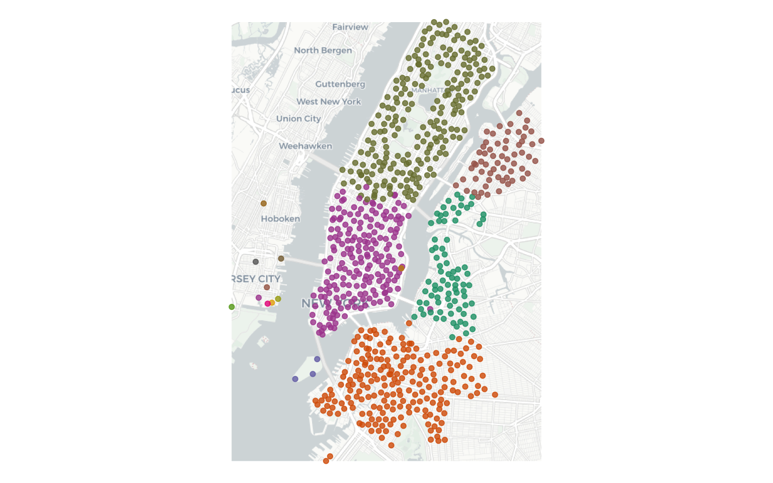
Community Detection
Finding a community structure in a network is to identify clusters of nodes that are more strongly connected within the cluster than to nodes outside the cluster. There are many algorithms that identify community structures. Some work on weighted networks and some work on digraphs. In any case it is better to convert multigraph (graph with two nodes having multiple edges) into a simple graph with edge weights, representing the number of trips.
E(trips_graph)$weight <- 1
station_graph  <- simplify(trips_graph, edge.attr.comb="sum")

ecount(station_graph) == ecount(trips_graph)
# [1] FALSE
sum(E(station_graph)$weight) == ecount(trips_graph)
# [1] TRUE
all.equal(vcount(station_graph), vcount(trips_graph))
# [1] TRUE

is.directed(station_graph)
# [1] TRUE
Walktrap algorithm finds the communities by random walks in the graph. The intuition is that random walks are more likely to be within a community that across communities.
wlktrp_mmbr <- data.frame (clstrmm  = cluster_walktrap(station_graph)$membership %>% as.factor,
                          stid = V(station_graph)$name %>% as.numeric()
                          ) %>% as.tibble()


wlktrp_mmbr$clstrmm %>% summary()
#   1   2   3   4   5   6   7   8   9  10  11  12  13  14  15
#  80 218 207  61   3 195   1   1   1   1   1   1   1   1   1
It seems like there are 5 distinct and non-trivial clusters of stations ($ n $). You can visualise these results by joining them back to tibbles with location information.
station_locs <- station_locs %>%
                inner_join(wlktrp_mmbr, by='stid')

library(basemaps)
library(RColorBrewer)
numColors <- levels(station_locs$clstrmm) %>% length()
myColors <- colorRampPalette(brewer.pal(8,"Dark2"))(numColors) # Expanding the number of colors available from 8

station_locs_shp <- st_as_sf(station_locs, coords = c("lon", 'lat'), crs = st_crs(4326))
ext <- station_locs_shp %>% st_bbox()


  ggplot()+
      basemap_gglayer(ext, map_type = 'light', map_service = 'carto')+
      scale_fill_identity()+
  geom_sf(data = station_locs_shp %>% st_transform(st_crs(3857)),
          aes(color = clstrmm), alpha = .8)+
  scale_color_manual(values = myColors)+
     scale_x_continuous("", breaks=NULL)+
   scale_y_continuous("", breaks=NULL)+
  labs(colour = "Communities", x = NULL, y = NULL) +
      labs(x=NULL, y=NULL) +
  theme(axis.line = element_blank(),  # Remove all the extraenous stuff from the plot.
        axis.text = element_blank(),
        axis.ticks = element_blank(),
        axis.title = element_blank(),
        axis.ticks.length = unit(0, "pt"), #length of tick marks
        legend.position = "none",
        panel.background = element_blank(),
        panel.border = element_blank(),
        panel.grid.major = element_blank(),
        panel.grid.minor = element_blank(),
        plot.background = element_blank(),
        plot.margin = unit(c(0,0,0,0),"mm"))
# Loading basemap 'light' from map service 'carto'...
# Using geom_raster() with maxpixels = 263341.
Exercise
- Use tmap instead of ggplot.
- Do the clusters change if you use a different algorithm?
- Are the clusters different for customers and subscribers? Men and Women?
- Are the clusters different at different times of the day? days of the week?
Conclusions
Network analysis techniques provide a very useful set of tools that we can apply in many contexts in urban analytics. Networks are ubiquitous and the above two are but few of the situations where network tools can be readily applied. They need to be used more, and used judiciously.
Nikhil Kaza
Professor
My research interests include urbanization patterns, local energy policy and equity