Transit Accessibility Using GTFS
Introduction
Understanding the reach and effectiveness of public transit is important to understand how urban environments are accessible for different groups of people. Analysing fixed route public transit has become relatively straightforward with the introduction of the “General Transit Feed Specification”, a common standard for transit agencies to publish their schedules. Pioneered by TriMet of Portland, Oregon in collaboration with Google, this specification has become common for transit agencies around the world to publish their consumer facing datasets.
GTFS is split into a schedule component that contains schedule, fare, and geographic transit information and a real-time component that contains arrival predictions, vehicle positions and service advisories. Static GTFS consists of routes, trips, stop_times, stops and calendar as mandatory tables. There are also other optional tables such as fares and frequencies. Real Time GTFS (gtfs-rt) consists of trip updates, service interruptions etc.
Reading in GTFS files
Because GTFS are regularly updated (usually semi-annually) and published on transit agency’s website, it is a good idea to get the latest schedule. Fortunately, Mobility Database has a catalogue of various GTFS feeds and their source locations. In this tutorial, I am going to use Metro St. Louis GTFS feed.
In addition, I am going to use tidytransit and gtfsrouter packages. extract_gtfs is a function in the gtfsrouter package that reads the zipfile and converts it into bunch of data tables. Similarly read_gtfs from tidytransit could also be used.
In the following code, I am showing how to download the latest GTFS files. However, I am going to use an archived GTFS files for consistency.
gtfs_feeds <- read_csv("https://bit.ly/catalogs-csv") %>%
               filter(provider == "Metro St. Louis") %>%
               filter(data_type == "gtfs") %>%
               pull('urls.direct_download')

gtfs_feeds


## function to download and read the gtfs feeds. Particularly helpful, if there are multiple feeds and/or multiple transit agencies in the area.

download_read_gtfs <- function(feed_url){
      zipfilename <- basename(feed_url)
     download.file(feed_url, destfile = zipfilename)
#      gtfsrouter::extract_gtfs(zipfilename)
      tidytransit::read_gtfs(zipfilename)
}

stlouis_gtfs <- gtfs_feeds %>% download_read_gtfs()

summary(stlouis_gtfs)
library(widgetframe)
library(tidytransit)
library(tidyverse)
library(sf)
library(units)
library(here)

stlouis_gtfs <- here("tutorials_datasets/gtfs/google_transit.zip") %>%tidytransit::read_gtfs()

summary(stlouis_gtfs)
# tidygtfs object
# files        agency, stops, routes, trips, stop_times, calendar, calendar_dates, shapes
# agency       Metro St. Louis
# service      from 2022-09-26 to 2023-03-12
# uses         stop_times (no frequencies)
# # routes       121
# # trips      17704
# # stop_ids    5315
# # stop_names  5256
# # shapes       420
Notice that there are about 121 routes with over 5,000 stops in the St. Louis region. Visualising these stops is pretty straightforward, once you convert them into sf objects.
stlouis_gtfs <- gtfs_as_sf(stlouis_gtfs, skip_shapes = FALSE, crs = 4326, quiet = TRUE)
stlouis_gtfs
# $agency
# # A tibble: 1 × 8
# agency_phone agency_url agenc…¹ agenc…² agenc…³ agenc…⁴ agenc…⁵ agenc…⁶
# <chr> <chr> <chr> <chr> <chr> <chr> <chr> <chr>
# 1 314-231-2345 http://www.metro… EN "" Metro … Americ… http:/… Transi…
# # … with abbreviated variable names ¹agency_lang, ²agency_id, ³agency_name,
# # ⁴agency_timezone, ⁵agency_fare_url, ⁶agency_email
#
# $calendar_dates
# # A tibble: 6 × 3
# service_id date exception_type
# <chr> <date> <int>
# 1 3_merged_3039412 2023-01-02 1
# 2 3_merged_3039412 2022-12-26 1
# 3 1_merged_3039411 2023-01-02 2
# 4 1_merged_3039411 2022-12-26 2
# 5 3_merged_3039415 2022-11-24 1
# 6 1_merged_3039414 2022-11-24 2
#
# $calendar
# # A tibble: 6 × 10
# service_id start_date end_date monday tuesday wedne…¹ thurs…² friday satur…³
# <chr> <date> <date> <int> <int> <int> <int> <int> <int>
# 1 2_merged_… 2022-09-26 2022-11-27 0 0 0 0 0 1
# 2 2_merged_… 2022-11-28 2023-03-12 0 0 0 0 0 1
# 3 3_merged_… 2022-11-28 2023-03-12 0 0 0 0 0 0
# 4 1_merged_… 2022-11-28 2023-03-12 1 1 1 1 1 0
# 5 3_merged_… 2022-09-26 2022-11-27 0 0 0 0 0 0
# 6 1_merged_… 2022-09-26 2022-11-27 1 1 1 1 1 0
# # … with 1 more variable: sunday <int>, and abbreviated variable names
# # ¹wednesday, ²thursday, ³saturday
#
# $stops
# Simple feature collection with 5315 features and 7 fields
# Geometry type: POINT
# Dimension: XY
# Bounding box: xmin: -90.66209 ymin: 38.46975 xmax: -89.87466 ymax: 38.82565
# Geodetic CRS: WGS 84
# # A tibble: 5,315 × 8
# wheelchair_boarding zone_id stop_id stop_desc stop_…¹ locat…² stop_…³
# * <int> <chr> <chr> <chr> <chr> <int> <chr>
# 1 2 "" 9160 FAR SIDE NATURAL… NATURA… 0 9160
# 2 2 "" 16079 FAR SIDE KINGSHI… KINGSH… 0 16079
# 3 2 "" 4446 FAR SIDE WOODSON… WOODSO… 0 4446
# 4 2 "" 5745 NEAR SIDE 546 NO… 546 NO… 0 5745
# 5 2 "" 16076 FAR SIDE CRAIG @… CRAIG … 0 16076
# 6 2 "" 16075 FAR SIDE CRAIG @… CRAIG … 0 16075
# 7 2 "" 16074 MID-BLOCK NATURA… NATURA… 0 16074
# 8 NA "" 11542 NEAR SIDE MEMORI… MEMORI… 0 11542
# 9 NA "" 11543 NEAR SIDE MEMORI… MEMORI… 0 11543
# 10 1 "" 4024 NEAR SIDE CHEROK… CHEROK… 0 4024
# # … with 5,305 more rows, 1 more variable: geometry <POINT [°]>, and
# # abbreviated variable names ¹stop_name, ²location_type, ³stop_code
#
# $routes
# # A tibble: 121 × 7
# route_long_name route…¹ route…² agenc…³ route…⁴ route…⁵ route…⁶
# <chr> <int> <chr> <chr> <chr> <chr> <chr>
# 1 MetroLink Red Line 2 f6f6fc "" 18164R CC0033 MLR
# 2 OFallon-Fairview Heights 3 000000 "" 18093 FFFFFF 12
# 3 Washington Park 3 000000 "" 18092 FFFFFF 9
# 4 Alta Sita 3 000000 "" 18091 FFFFFF 8
# 5 Rosemont 3 000000 "" 18090 FFFFFF 6
# 6 St Clair Square 3 000000 "" 18097 FFFFFF 16
# 7 Belleville-Shiloh-OFallon 3 000000 "" 18096 FFFFFF 15
# 8 Memorial Hosp-Westfield Plaza 3 000000 "" 18095 FFFFFF 14
# 9 Caseyville-Marybelle 3 000000 "" 18094 FFFFFF 13
# 10 OFallon-Fairview Heights 3 000000 "" 18158 FFFFFF 12
# # … with 111 more rows, and abbreviated variable names ¹route_type,
# # ²route_text_color, ³agency_id, ⁴route_id, ⁵route_color, ⁶route_short_name
#
# $trips
# # A tibble: 17,704 × 8
# block_id route_id wheelchair_access…¹ direc…² trip_…³ shape…⁴ servi…⁵ trip_id
# <chr> <chr> <int> <int> <chr> <chr> <chr> <chr>
# 1 b_65655 18076 1 0 TO NOR… 110261 2_merg… 3020482
# 2 b_65657 18076 1 0 TO NOR… 110261 2_merg… 3020483
# 3 b_65655 18076 1 0 TO NOR… 110261 2_merg… 3020480
# 4 b_65654 18076 1 0 TO NOR… 110261 2_merg… 3020481
# 5 b_65657 18076 1 0 TO NOR… 110261 2_merg… 3020486
# 6 b_65657 18076 1 0 TO NOR… 110261 2_merg… 3020487
# 7 b_65657 18076 1 0 TO NOR… 110261 2_merg… 3020484
# 8 b_65656 18076 1 0 TO NOR… 110261 2_merg… 3020485
# 9 b_65656 18076 1 0 TO NOR… 110261 2_merg… 3020488
# 10 b_65652 18076 1 0 TO NOR… 110259 2_merg… 3020489
# # … with 17,694 more rows, and abbreviated variable names
# # ¹wheelchair_accessible, ²direction_id, ³trip_headsign, ⁴shape_id,
# # ⁵service_id
#
# $stop_times
# # A tibble: 945,643 × 10
# trip_id arrival_time depart…¹ stop_id stop_…² stop_…³ picku…⁴ drop_…⁵ shape…⁶
# <chr> <time> <time> <chr> <int> <chr> <int> <int> <dbl>
# 1 3020482 16:50 16:50 16146 1 "" NA NA NA
# 2 3020482 16:51 16:51 16301 2 "" NA NA 677.
# 3 3020482 16:51 16:51 16281 3 "" NA NA 1000.
# 4 3020482 16:52 16:52 10164 4 "" NA NA 1574.
# 5 3020482 16:54 16:54 15534 5 "" NA NA 2670.
# 6 3020482 16:55 16:55 14708 6 "" NA NA 3301.
# 7 3020482 16:56 16:56 6691 7 "" NA NA 3866.
# 8 3020482 16:57 16:57 6693 8 "" NA NA 4196.
# 9 3020482 16:57 16:57 6694 9 "" NA NA 4474.
# 10 3020482 16:58 16:58 6695 10 "" NA NA 4836.
# # … with 945,633 more rows, 1 more variable: timepoint <int>, and abbreviated
# # variable names ¹departure_time, ²stop_sequence, ³stop_headsign,
# # ⁴pickup_type, ⁵drop_off_type, ⁶shape_dist_traveled
#
# $shapes
# Simple feature collection with 420 features and 1 field
# Geometry type: LINESTRING
# Dimension: XY
# Bounding box: xmin: -90.66385 ymin: 38.4682 xmax: -89.87396 ymax: 38.82576
# Geodetic CRS: WGS 84
# First 10 features:
# shape_id geometry
# 1 110120 LINESTRING (-90.30889 38.64...
# 2 110121 LINESTRING (-90.30062 38.65...
# 3 110122 LINESTRING (-90.2599 38.635...
# 4 110124 LINESTRING (-90.30172 38.68...
# 5 110125 LINESTRING (-90.30172 38.68...
# 6 110126 LINESTRING (-90.30172 38.68...
# 7 110129 LINESTRING (-90.33777 38.62...
# 8 110131 LINESTRING (-90.30814 38.64...
# 9 110132 LINESTRING (-90.315 38.7197...
# 10 110134 LINESTRING (-90.20271 38.62...
#
# $.
# $.$dates_services
# # A tibble: 168 × 2
# date service_id
# <date> <chr>
# 1 2022-09-26 1_merged_3039414
# 2 2022-09-27 1_merged_3039414
# 3 2022-09-28 1_merged_3039414
# 4 2022-09-29 1_merged_3039414
# 5 2022-09-30 1_merged_3039414
# 6 2022-10-01 2_merged_3039416
# 7 2022-10-02 3_merged_3039415
# 8 2022-10-03 1_merged_3039414
# 9 2022-10-04 1_merged_3039414
# 10 2022-10-05 1_merged_3039414
# # … with 158 more rows
library(tmap)
tmap_mode("view")
m1 <- tm_shape(stlouis_gtfs$stops)+
tm_dots(col = "red")+
tm_shape(stlouis_gtfs$shapes) +
tm_lines(col = 'green', alpha = 0.5)+
tm_basemap(leaflet::providers$Stamen.Toner)
library(widgetframe)
frameWidget(tmap_leaflet(m1))
Analysing Service Patterns
The GTFS reference specifies that a “service_id contains an ID that uniquely identifies a set of dates when service is available for one or more routes”. A service could run on every weekday or only on Saturdays for example. However, feeds are not required to indicate anything with service_ids and some feeds even use a unique service_id for each trip and day. Service patterns can be used to find a typical day for further analysis like routing or trip frequencies for different days.
stlouis_gtfs <- set_servicepattern(stlouis_gtfs)

# service ids used
length(unique(stlouis_gtfs$trips$service_id))
# [1] 6

# unique date patterns
length(unique(stlouis_gtfs$.$servicepatterns$servicepattern_id))
# [1] 6
In this particular instance, service patterns and service_ids are the same.
#Visualise the service patterns.

calendar <- tibble(date = unique(stlouis_gtfs$.$dates_services$date)) %>%
  mutate(
    weekday = (function(date) {
      c("Sunday", "Monday", "Tuesday",
        "Wednesday", "Thursday", "Friday",
        "Saturday")[as.POSIXlt(date)$wday + 1]
    })(date)
  )

stlouis_gtfs$.$dates_servicepatterns %>%
  left_join(calendar, by = 'date') %>%
  ggplot()+
  geom_point(aes(x = date, y = servicepattern_id, color = weekday), size = 1) +
  scale_x_date(breaks = scales::date_breaks("1 month")) + theme(legend.position = "bottom")
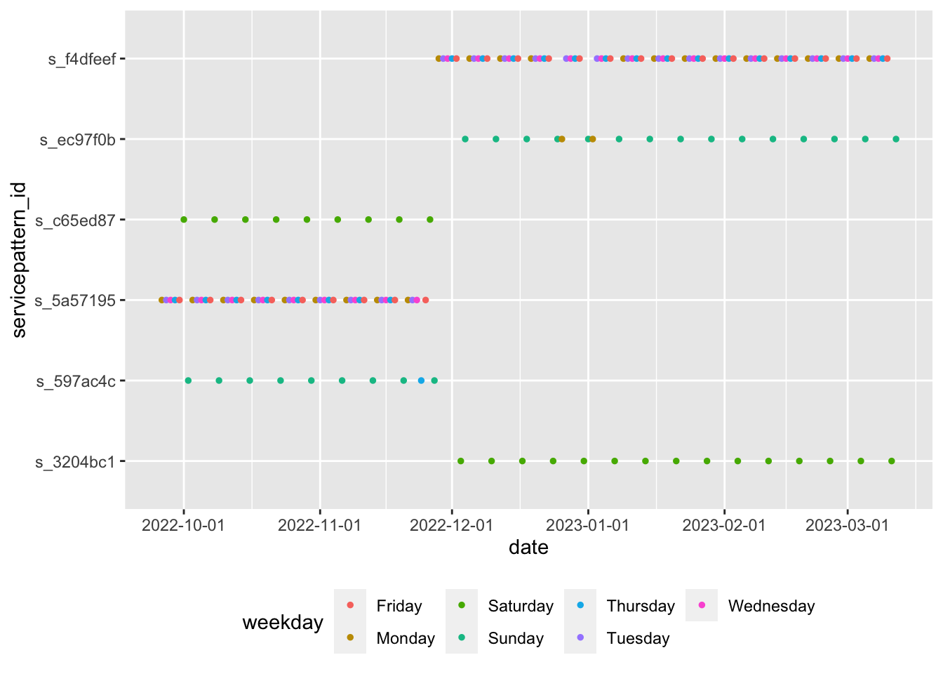
The above figure shows that s_3204bc1 service pattern is a Saturday service from Dec 2022, while s_597ac4c is mostly a Saturday service with occasional Thursday before Dec 2022. s_5a57195 and s_f4dfeef seem to be weekday service patterns. We use those service patterns to calculate the frequencies for the rest of the tutorial.
service_ids <- stlouis_gtfs$.$servicepattern %>%
  filter(servicepattern_id %in%  c('s_5a57195', 's_f4dfeef' )) %>%
  pull(service_id)
Getting route frequncies are straightforward when we know which service patterns we want to use. tidytransit uses times as seconds from the midnight. If we want midday frequency between 11 AM and 4 PM, we need to convert them to seconds.
Please pay explicit attention to the units and their conversion, as I have done below.
midday_route_freq <- get_route_frequency(stlouis_gtfs, service_ids = service_ids,
                                     start_time = 11*3600, end_time = 16*3600) %>% # these are in seconds starting from 00H00.
                       mutate(across(ends_with("headways"),  ~units::set_units(.x, 's'))) %>%
                       mutate(across(ends_with("headways"),  ~units::set_units(.x, 'min')))


m1 <-
get_route_geometry(stlouis_gtfs, service_ids = service_ids) %>%
  inner_join(midday_route_freq, by = "route_id") %>%
  mutate(frequency = (1/set_units(median_headways, "hr"))) %>%
  tm_shape()+
  tm_lines(col='frequency', alpha = 0.4, style = "pretty", n=4, scale = 5, lwd = "frequency") +
  tm_basemap(leaflet::providers$Stamen.Toner)

frameWidget(tmap_leaflet(m1))
While it is fine to know which routes are more frequent than others, it is also useful to know which stops have smaller headways and more frequent departures.
midday_stops <-
  get_stop_frequency(stlouis_gtfs, start_time = 11*3600, end_time = 16*3600, # these are in seconds starting from 00H00.
                              service_ids = service_ids, by_route = FALSE) %>%
  mutate(mean_headway = units::set_units(mean_headway, "s"),
         mean_headway  = units::set_units(mean_headway, "min")) %>%
  arrange(mean_headway)
Notice that stop frequencies are summarised by different service patterns. Since we selected multiple patterns, we need to average them out to get a reasonable estimate.
midday_stops_summ <- midday_stops %>%
group_by(stop_id) %>%
  summarise(n_departures = sum(n_departures, na.rm = T),
            mean_headway = mean(mean_headway, na.rm=T)) %>%
  arrange(mean_headway)

head(midday_stops_summ)  # Some stops have less than 3 min wait time. However, note that this is not by route, because we set the argument in such a way in earlier piece of code
# # A tibble: 6 × 3
#   stop_id n_departures mean_headway
#   <chr>          <int>        [min]
# 1 13330            199         3.02
# 2 14330            184         3.27
# 3 14769            165         3.64
# 4 11102            160         3.75
# 5 14792            160         3.75
# 6 7424             142         4.23

tail(midday_stops_summ)  # Some stops have more than 2 hr wait between the buses
# # A tibble: 6 × 3
#   stop_id n_departures mean_headway
#   <chr>          <int>        [min]
# 1 16085              6         112.
# 2 13653              4         150
# 3 16293              4         150
# 4 6086               4         150
# 5 15619              3         225
# 6 13966              2         300

m1 <-
stlouis_gtfs$stops %>%
 left_join(midday_stops_summ, by='stop_id') %>%
 mutate(bubble_size = n_departures^2) %>%
 tm_shape()+
 tm_dots(size = "bubble_size", style = "cont", alpha=.7, popup.vars = "stop_name", id = 'stop_name') +
 tm_shape(stlouis_gtfs$shapes)+
 tm_lines(col = 'green', alpha =.1) +
 tm_basemap(leaflet::providers$Stamen.Toner)

frameWidget(tmap_leaflet(m1))
Notice how some stops have more frequent departures and some have long wait times. There are some spatial patterns. The classic hub and spoke transit system means that the downtown (hub) have a lot of stops that have high quality transit. However, there are also some transit centers at the outskirts that also have large number of departures. These serve as transfer stations or terminus.
Exercise
-
Notice that these stop frequencies do not account for routes. However, it may be more useful to get the frequencies averaged by the route. Does the geography of access change?
-
In the above, only midday weekday services are mapped out. What about other patterns? Saturday Morning might have a different accessibility pattern. Think about how to analyse them and represent the variation over day as well as over the week.
-
If there are seasonal variations, it would be helpful to know. For example, university transit systems have reduced operations during Winter and Summer breaks. Using the above as a template, and Duke University transit as your public transit system, figure out the seasonal variations in accessibility.
Accessibility as Cumulative Opportunity
While it is useful to think of accessibility as frequency of transit at a particular location, that indicator does not tell us much about the system level accessibility. While a specific bus station might have frequent departures, it may be on a line that is broadly disconnected from the rest of the transit system (e.g. connected to other lines that have significant wait times). It is thus useful to measure accessibility as opportunities that can be accessed within a travel budget (say 45 minutes). To do compute these, it is useful to figure out how much area can be covered within 45 min of travel time.
It is reasonably straightforward to figure out how much area can be covered by foot using routing engines such as OSRM. The tricky bit is to figure out how much time is spent waiting at transit stations before boarding the buses/trains and during transfers.
Typically, accessibility is measured for centroids of population centers (block groups e.g.). However, any origin set should be fine. I select the the three counties for the analysis (St. Clair in IL and St. Louis City, St. Louis County in MO)
transitstops <- stlouis_gtfs$stops

blkgrp_centroid <- list()

blkgrp_centroid[[1]] <- tigris::block_groups(state="MO", county = c('510', '189'), progress_bar = FALSE) %>%
                        st_centroid() %>%
                        st_transform(st_crs(transitstops)) %>%
                        select(GEOID)

blkgrp_centroid[[2]] <- tigris::block_groups(state="IL", county = '163', progress_bar = FALSE) %>%
  st_centroid() %>%
  st_transform(st_crs(transitstops)) %>%
  select(GEOID)


blkgrps <- do.call(rbind, blkgrp_centroid)
An analytical decision to make early on is to assign the origin to a nearest starting point on the transit network or to the nearest starting point on the road (foot/bike) network. It is always more computationally expensive to model both the first and last mile of travel. In this tutorial, I will demonstrate how this might be possible.
We need to operationalise a few things. Some of them are easier to precompute and some of them are easier on the fly.
-
Travel time from each origin (block group centroid) to each destination (transit station) by foot. This is presumably time invariant, as the road network is not subject to schedules. However, this is highly dependent on the quality of the road network and appropriate information about crossings and non-pedestrian roads.
-
Travel time from each transit station to every other transit station. For the sake of practicality, we will limit the number of transfers to 3. This is highly dependent on schedules, especially when the trip starts and what time the transit reaches each stop and if there are any transfers available to other routes within the travel budget. This is time varying.
-
The geography that can be covered from each transit stop in the remaining time after the transit trip is concluded. While, we do not know apriori how much time is remaining, we know that it cannot exceed the travel budget (45 min). So we can precompute 1 min ischocrones from each transit station and select them as necessary.
-
While we are focused on transit, it could very well be that many of the blockgroups may not have access to good quality transit and therefore the entire travel budget is spent on foot.Thus, we also compute the isochrones for the blockgroup centeroids.
All the steps (except the second) can be computed using routing engines such as OSRM. Since these are time consuming, I am only going to show the code rather than running it. For this to run, OSRM needs to be set up with appropriate street networks. See
library(osrm)

options(osrm.server = "http://localhost:5000/")
options(osrm.profile = 'foot')


ttmatrix <- osrmTable(src=blkgrps, dst=transitstops, measure = c('duration'))
ttmatrix$durations <- round(ttmatrix$durations)

stop_iso <- list()
stop_iso <- map(1:nrow(transitstops), possibly(function(x){osrmIsochrone(loc=transitstops[x,], breaks = seq(0,45,1))}, otherwise = NULL))

blkgrp_iso <- list()
blkgrp_iso <- map(1:nrow(blkgrps), possibly(function(x){osrmIsochrone(loc=blkgrps[x,], breaks = seq(0,45,1))}, otherwise = NULL))
I precomputed these and saved them in an RData file. The RData file has three main objects. stop_iso is list of isochrones for each stop. blkgrp_iso is the list of isochrones for each blkgrp. ttmatrix is large list where the element duration is a travel time matrix from blkgrps to transit stops.
Some clean up is necessary, like adding names to easily filter and identify.
load(here::here("tutorials_datasets/gtfs/ttmatrix.RData"))

str(blkgrp_iso[[1]])
# Classes 'sf' and 'data.frame':    42 obs. of  4 variables:
#  $ id      : int  1 2 3 4 5 6 7 8 9 10 ...
#  $ isomin  : num  0 4 5 6 7 8 9 10 11 12 ...
#  $ isomax  : num  4 5 6 7 8 9 10 11 12 13 ...
#  $ geometry:sfc_MULTIPOLYGON of length 42; first list element: List of 1
#   ..$ :List of 1
#   .. ..$ : num [1:7, 1:2] -90.2 -90.2 -90.2 -90.2 -90.2 ...
#   ..- attr(*, "class")= chr [1:3] "XY" "MULTIPOLYGON" "sfg"
#  - attr(*, "sf_column")= chr "geometry"
#  - attr(*, "agr")= Factor w/ 3 levels "constant","aggregate",..: NA NA NA
#   ..- attr(*, "names")= chr [1:3] "id" "isomin" "isomax"
length(blkgrp_iso)
# [1] 1260

str(stop_iso[[1]])
# Classes 'sf' and 'data.frame':    41 obs. of  4 variables:
#  $ id      : int  1 2 3 4 5 6 7 8 9 10 ...
#  $ isomin  : num  0 5 6 7 8 9 10 11 12 13 ...
#  $ isomax  : num  5 6 7 8 9 10 11 12 13 14 ...
#  $ geometry:sfc_MULTIPOLYGON of length 41; first list element: List of 1
#   ..$ :List of 1
#   .. ..$ : num [1:7, 1:2] -90.3 -90.3 -90.3 -90.3 -90.3 ...
#   ..- attr(*, "class")= chr [1:3] "XY" "MULTIPOLYGON" "sfg"
#  - attr(*, "sf_column")= chr "geometry"
#  - attr(*, "agr")= Factor w/ 3 levels "constant","aggregate",..: NA NA NA
#   ..- attr(*, "names")= chr [1:3] "id" "isomin" "isomax"
length(stop_iso)
# [1] 5315

str(ttmatrix)
# List of 3
#  $ durations   : num [1:1260, 1:5315] 208 191 186 180 186 217 195 190 92 178 ...
#   ..- attr(*, "dimnames")=List of 2
#   .. ..$ : chr [1:1260] "1" "2" "3" "11" ...
#   .. ..$ : chr [1:5315] "1" "2" "3" "4" ...
#  $ sources     :'data.frame': 1260 obs. of  2 variables:
#   ..$ lon: num [1:1260] -90.2 -90.2 -90.2 -90.4 -90.4 ...
#   ..$ lat: num [1:1260] 38.8 38.8 38.8 38.8 38.8 ...
#  $ destinations:'data.frame': 5315 obs. of  2 variables:
#   ..$ lon: num [1:5315] -90.3 -90.3 -90.4 -90.3 -90.4 ...
#   ..$ lat: num [1:5315] 38.7 38.6 38.7 38.8 38.7 ...

row.names(ttmatrix$durations) <-  blkgrps$GEOID

plot(blkgrp_iso[[4]][5,"id"])

Based on the above, it looks likes each element of the isochrone list corresponds to either origin or destination. Each of that element is a tibble with isomin and isomax times (e.g. can be reached between 10 and 11 min). But we need the cumulative isochrone (e.g. reached within 11 min) for stops and only 45 min isochrone from block groups.
sf_use_s2(FALSE)

names(stop_iso) <- stlouis_gtfs$stops$stop_id
stop_iso_cumulative <- map(stop_iso, ~nngeo::st_remove_holes(.))

names(blkgrp_iso) <- blkgrps$GEOID
blkgrp_iso_cumulative <- map(blkgrp_iso,
                            ~ slice_max(., isomax, n = 1) %>%
                              nngeo::st_remove_holes() %>%
                              st_geometry() %>%
                              st_make_valid()
                            )

# We don't need the attributes for the block group isochrones any more (they are all 45 min) so we only keep that geometry.
The second part is computed using the Round-Based Public Transit Routing Algorithm (RAPTOR) for each start time. But first we need to make a transfer table. Typically GTFS should come with one that specifies the time taken to transfer between two stations (within reasonable time frame). Since we do not have it here in the St. Louis GTFS, we infer one based on distance (typically within 200 m). We need the gtfsrouter package for this.
But first we must recover stop_lon and stop_lat in the stops table that we lost when we converted using gtfs_as_sf.
stlouis_gtfs$stops <- stlouis_gtfs$stops %>%
  bind_cols(st_coordinates(stlouis_gtfs$stops)) %>%
  rename(stop_lon = X, stop_lat = Y)

stlouis_gtfs$transfers <-
  gtfsrouter::gtfs_transfer_table(stlouis_gtfs)
In the following code, I am going to demonstrate the extent of reach for a single block group “291892138006” and focus on the variation through out the day on a weekday. Let’s focus on a single start time at 6:20 AM and then figure out how to iterate over a vector of times and blkgrops
library(lubridate)

blk_start_time <- "6:20" %>% hm %>% period_to_seconds
blkgrp_id <- "291892138006"

geo_temp_sf2 <- blkgrp_iso_cumulative[[blkgrp_id]]


# The following computes how much time it takes to reach different transit stations from the block group centeroid and how much time is leftover in the travel budget that can be used for waiting/transit travel.

travel_to_stations <-
        tibble(tt = ttmatrix$durations[blkgrp_id,],
               stop_id = stlouis_gtfs$stops$stop_id) %>%
        filter(tt <= 45) %>%  # Note that these are in minutes rather than seconds.
        mutate(min_start_time = blk_start_time + tt * 60,
               max_start_time = blk_start_time + 45 * 60,
               allowed_timerange = max_start_time - min_start_time) %>%
        filter(allowed_timerange >0)


##  The following code calculates for each transit station that can be accessed by foot with 45 min, the other transit stations that can be accessed by transit and the remaining time from travel budget.

remain_time_dt <- map_dfr(1:nrow(travel_to_stations), function(idx) {
  transit_stop_times <- filter_stop_times(stlouis_gtfs, "2022-11-22",
                                          min_departure_time = travel_to_stations[idx,] %>% pull("min_start_time"))

  raptor(
    transit_stop_times,
    stlouis_gtfs$transfers,
    stop_ids = travel_to_stations[idx,] %>% pull('stop_id'),
    time_range = travel_to_stations[idx, ] %>% pull('allowed_timerange'),
    max_transfers = 3,
    keep = 'shortest'
  )
}) %>%
  mutate(remain_time = (blk_start_time + 45 * 60) - journey_arrival_time) %>%
  filter(remain_time >0) %>%
  select(to_stop_id, remain_time) %>%
  bind_cols(tibble("GEOID" = blkgrp_id, "start" = blk_start_time))


# For each reachable transit stop, extract the isochrone that is corresponding to the remaining travel time on the budget.

geo_temp_sf1 <-
  map_dfr(1:nrow(remain_time_dt), function(idx) {
    stop_iso_cumulative[[remain_time_dt[idx, ]$to_stop_id]] %>%
      filter(isomax <= remain_time_dt[idx, ]$remain_time / 60) %>%
      slice_max(isomax, n = 1)
  }) %>%
  st_union() %>%
  st_make_valid()


## Union the various polygons along with the foot isochrone of the block group.
geo_sf <-
  st_union(geo_temp_sf2, geo_temp_sf1)  %>%
  st_sf(GEOID = blkgrp_id, start = blk_start_time) %>%
  st_make_valid()


m1 <-
  tm_shape(geo_sf) +
  tm_polygons(col = 'blue', alpha = .5) +
  tm_shape(blkgrps %>% filter (GEOID == blkgrp_id)) +
  tm_markers() +
  tm_basemap(leaflet::providers$Stamen.Toner)

frameWidget(tmap_leaflet(m1))
Exercise
-
Create a function that will take start time as an argument and return the transit+walk isochrones for a block group. Use it to compute the isochrones for every 10 min for a single block group
-
Create a function that will return the isochrones for a single start time, but for all block groups.
-
Combine the two functions and create the isochrones that change over time and over space for all of St. Louis. What story can you tell about diurnal variation in accessibility.
-
Repeat this exercise for a transit system that has significant weekly and seasonal variablity (e.g. Duke/Durham)
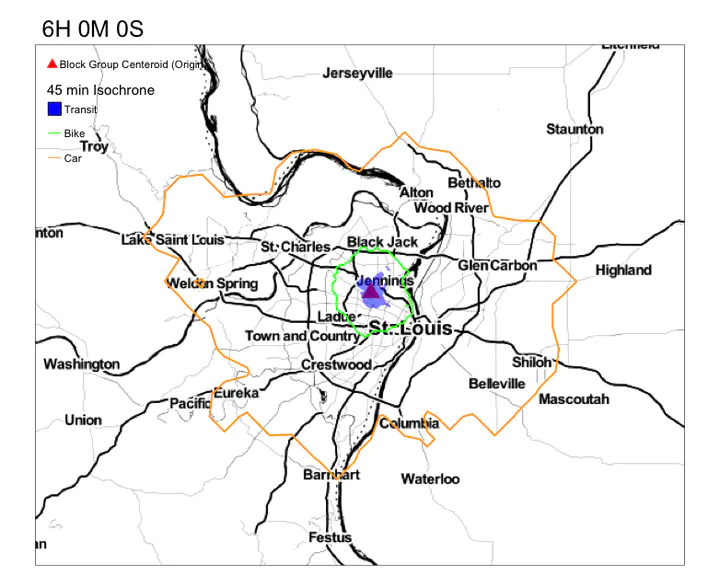
Your goal is to get something that resembles this.
Notice the variation in the reacheable area by transit in 45 min. Compare that to the reacheable areas by biking and driving.
Conclusions
Cumulative Opportunity is only one type of accessibility measures and perhaps not even the most useful one. But the above code can be easily adapted to gravity based measures or even any other kind of time/distance decay weighting. In any case, it is important to recognise that accessibility is unevenly distributed in both space and in time. Cumulative Opportunity is as good as any in demonstrating this.
Also while GTFS is about schedules, it is important to note that real travel times on transit systems rarely conform to the schedule. It is useful to think about how real time information can be useful in understanding why transit may or may not be a viable option for different constraints of life. More importantly, the above analysis does not account for tours and has implicitly assumed trips as the basis for accessibility. Again, caution should be used to interpret these.
Nikhil Kaza
Professor
My research interests include urbanization patterns, local energy policy and equity