Isochrones from Routing Engines (OSRM)

Introduction

In other posts, I have shown how to use external servers (google, craigslist etc.) to access information. You can also query a local (on your computer) server and your R session acts like a client (e.g. browser).

We can demonstrate this using (Open Source Routing Machine) OSRM server and constructing Isocrhrones. Isochrones are area you can reach from a point within a specified time. Often isochrones are used to identify gaps in the service area boundaries (e.g. 15 min distance from fire stations).

We can plot isochornes of every 2 min biking, around some random points in Orange County, NC. While we use OSRM, though any other API works as well (e.g. Google, Mapbox etc. see this blog for example.) . If you want to set other types of local routing engine, Valhalla and associated R packages might be a good option. Use whichever one suits your needs.

Setting up a OSRM server

We are going to set up a OSRM server on your computer.

• Different OS require different instructions, so please follow the website to construct the backend for your OS.

• Download North Carolina road network from Openstreetmap from Geofabrik for example (use the pbf file).

• Construct a graph that can be used for finding shortest routes. Use suitably modified versions of (mind the file locations)

    - osrm-extract nc.osm.pbf -p ./profiles/bicycle.lua
    - osrm-partition nc.osrm
    - osrm-customize nc.osrm
    - osrm-routed --algorithm mld nc.osrm 

in the command window/terminal (outside R). If all goes well, this sequence of steps will create local server ready to accept your requests. The server will be ready to be queried at http://localhost:5000/ or http://127.0.0.1:5000

To get other modes, simply change the lua profile.

The following code is here for the sake of completeness and is not evaluated. it can only be evaluated with the server is runnign in the background at localhost:5000

library(osrm)
library(tidyverse)
library(sf)
library(leaflet)
library(widgetframe)

# Ideally set these options up
 options(osrm.server = "http://localhost:5000/")
options(osrm.profile = 'bike') 

randompoints <- matrix(c( -79.065443, 35.924787, -79.087353, 35.914525, -79.066203, 35.881521), 
                       ncol=2, byrow =TRUE) %>%
                      data.frame()
names(randompoints) <- c('lng', 'lat')
randompoints$name <- c('pt1', 'pt2', 'pt3')

rt <- osrmRoute(src = randompoints[1,c('name', 'lng','lat')], 
                dst = randompoints[2,c('name','lng','lat')], 
                returnclass = "sf")

m1 <- 
rt %>% leaflet() %>%
    addProviderTiles(providers$Stamen.TonerLines, group = "Basemap") %>%
  addProviderTiles(providers$Stamen.TonerLite, group = "Basemap") %>%
  addMarkers(data=randompoints[1:2,], ~lng, ~lat) %>%
  addPolylines(weight =5, smoothFactor = .5, color='red')


frameWidget(m1)

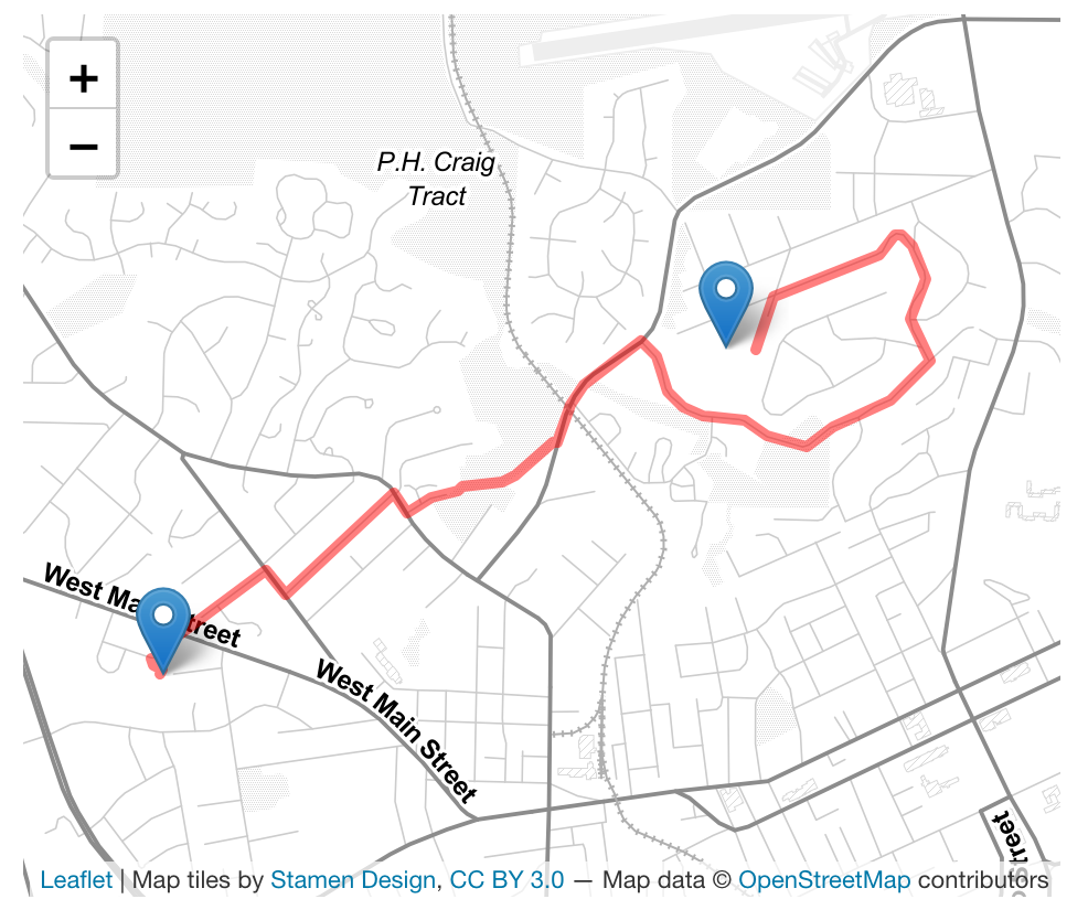
OSRM is a convenience package that is wrapping the calls to the server and parsing the output into sf classes. For example, the curl query in the backend looks like

http://localhost:5000/route/v1/biking/-78.901330,36.002806,-78.909020,36.040266

and should result in the following image

You can always shut the server down by closing the terminal/command window, after you are done with your analysis.

To get a matrix of distances and durations between multiple points,

ttmatrix <- osrmTable(loc=randompoints[, c('name', 'lng', 'lat')], measure = c('duration', 'distance'))

ttmatrix$durations should return a table similar to

	pt1	pt2	pt3
pt1	0.0	22.8	32.5
pt2	22.8	0.0	25.1
pt3	32.9	25.8	0.0

Querying a OSRM server

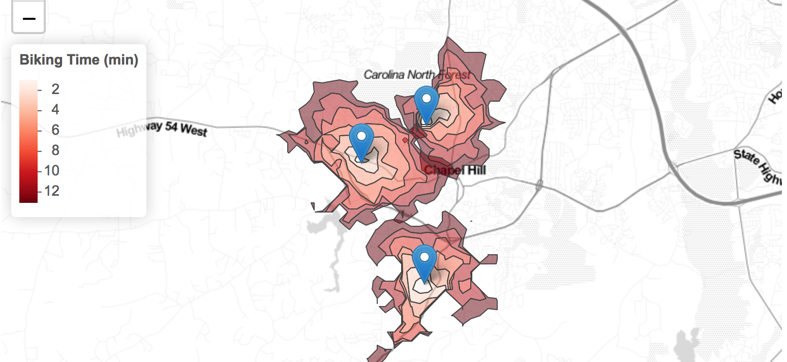
iso <- list()
for (i in 1:nrow(randompoints)){
iso[[i]] <- osrmIsochrone(loc = randompoints[i,c('lng','lat')], breaks = seq(from = 0,to = 15, by = 2)) %>% st_as_sf()
}

iso <- do.call('rbind', iso)

 Npal <- colorNumeric(
   palette = "Reds", n = 5,
   domain = iso$center
 )
 
iso %>% leaflet() %>%
  addProviderTiles(providers$Stamen.TonerLines, group = "Basemap") %>%
  addProviderTiles(providers$Stamen.TonerLite, group = "Basemap") %>%
  addMarkers(data=randompoints, ~lng, ~lat) %>%
  addPolygons(color = "#444444", weight = 1, smoothFactor = 0.5,
    opacity = 1.0, fillOpacity = 0.5, fillColor = ~Npal(iso$center),
    group = "Isochrone") %>%
  addLegend("topleft", pal = Npal, values = ~iso$center,
            title = "Biking Time (min)",opacity = 1
            )

The result should looks similar to the following.

---

Exercise

• Change the profile of the OSRM server to car and notice the differences in the Isochrones (shapes and extents).
• Repeat the entire exercise for all the major shopping areas in the Triangle.

---

Conclusions

It should be obvious that having a local server might reduce latency and allow for quicker turnaround. However, there are some distinct disadvantages compared to commercial option, including but not limited to incorporating real time information, setup costs and maintenance costs. Nonetheless, it is useful to think about how these might be beneficial within an organisation.