Object Detection Using Pre-trained Neural Network Models
Introduction
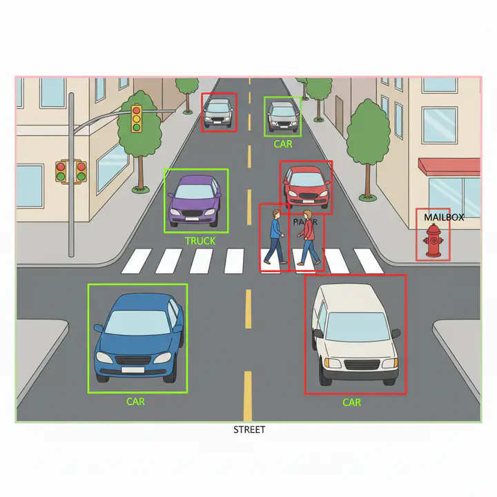
Object detection allows computers to identify and locate objects — like cars, people, street furniture — in images or videos. For urban planners, it offers a way to gather observational data at scale.
It can be used in various applications such as
- Traffic and Mobility Studies: Count vehicles, bikes, or pedestrians at intersections to inform signal timing or street design.
- Public Space Monitoring: Understand how parks, plazas, or transit stops are used throughout the day.
- Infrastructure Audits: Use aerial or street-level imagery to assess curb usage, sidewalk conditions, or construction activity.
Often these are meant to be supplement human data collection, but come with their own caveats. More on that later.
Often object detection uses deep learning, though other computer vision tools are occasionally used. Deep learning is a techniques that uses neural networks that are ‘deep’ (multiple layers) as opposed to a shallow single layer networks. Neural networks are a type of computer model inspired by how the human brain works — they learn patterns from data and use that knowledge to make predictions or recognize things.
They require enormous amount of training data. One of the most widely used datasets for training these models is the COCO dataset (Common Objects in Context), which contains thousands of labeled images featuring everyday scenes with people, vehicles, animals, and more. Because training a neural network from scratch requires a lot of data and computing power, we often use pretrained models — models that have already been trained on datasets like COCO — and then fine-tune them for specific tasks or environments. This makes it easier and faster to apply object detection in real-world settings, including urban planning, without needing to build everything from the ground up.
In this tutorial, we will explore how to use pre-trained neural network models for object detection using R. We will not do any fine tuning as this is meant as an illustration.
Data
For this tutorial, we will use street-level images from Rio de Janeiro, Brazil, available through Kartaview is an open-source platform for collecting and sharing street-level imagery, similar to Google Street View but built by a global community. It allows users to upload images captured from smartphones or dash cams, which can then be used for mapping, navigation, and research. You can download the images and unzip them into your InputData folder.
library(here)
library(magick)
library(tidyverse)

img_files <- here("tutorials_datasets", "rio_kartaview_images", "geotagged") %>%  #suitably modify the file path
              list.files(full.names = TRUE, pattern = "\\.jpg$") # Note the use of regular expressions to only load jpg file paths.
Let’s view a few random images first to visually inspect some. I am going to use magick and cowplot packages to read and plot the images
library(cowplot)

set.seed(123)

plot_list <- sample(img_files, 10) %>% # Randomly sample 10 image file paths
                map(function(x) {
                  image_read(x) %>%  ## This is a function from magick package. Read the image
                    image_ggplot() + ## This is a function from magick package. Convert the image to a ggplot object
                    theme_void() ## Note the switch between %>% and +. The former is for chaining functions, the latter is for adding layers to ggplot. This removes the axes and background.
                })

plot_grid(plotlist = plot_list, nrow = 2, ncol = 5) #plot_grid is a layout function from cowplot package to arrange multiple ggplot objects in a grid.
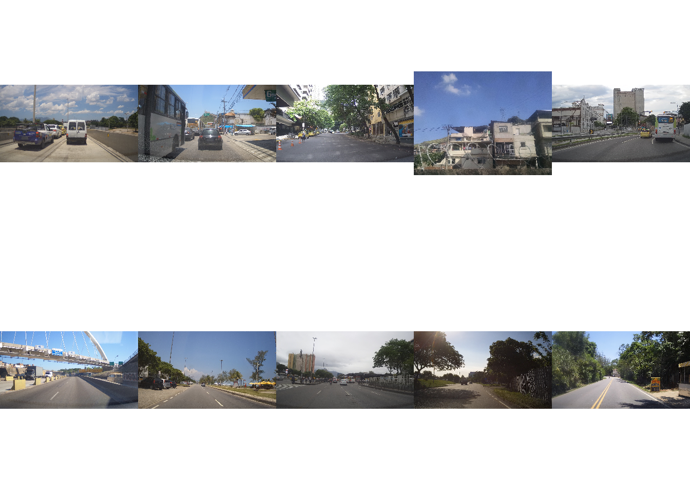
Note the variation in lighting conditions, angles, zoom levels, focus and occlusions. This is typical of street-level imagery and can pose challenges for object detection models. Also note the differences in urban settings such as highway, commercial corridor, vegetation cover etc.
In addition to data within the images, it is useful to look at the metadata associated with the images. In the case of images, metadata can include details such as the date and time the photo was taken, camera type, the camera settings used, the geographic location (latitude and longitude) where the image was captured. EXIF (Exchangeable Image File Format) is a standard that stores metadata within image files. This information is automatically recorded by most digital cameras and smartphones and we can use the exiftoolr package to extract this information. exiftoolr requires exiftool to be installed on your computer . You can find instructions here or uncomment appropriate line in the code.
library(exiftoolr)
# install_exiftool() # Uncomment this line if you don't have exiftool installed already.

img_metadata <- sample(img_files, 10) %>%
                exif_read() %>%
                  select(FileName,ImageWidth, ImageHeight, Megapixels, GPSLatitude, GPSLongitude)

head(img_metadata)
#                                      FileName ImageWidth ImageHeight Megapixels
# 1           330665659__1308095_016b5_5175.jpg       3072        1728   5.308416
# 2 1318418389__3645437_4e431_60c0edf80bea9.jpg       3232        2424   7.834368
# 3           346918433__1323919_5d1ab_1179.jpg       3072        1728   5.308416
# 4             325991853__1305043_cfec6_97.jpg       3072        1728   5.308416
# 5 1320102509__3654977_2dea0_60c23cb128f9f.jpg       3840        2160   8.294400
# 6             204024303__1129811_162e7_50.jpg       2340        4160   9.734400
#   GPSLatitude GPSLongitude
# 1   -22.91927    -43.25491
# 2   -22.86169    -43.30698
# 3   -22.81576    -43.30089
# 4   -22.89630    -43.19573
# 5   -22.97323    -43.39293
# 6   -22.89879    -43.10323
Exercise
- Visualise the locations of all images. Note any patterns you see in the spatial distribution of images. Does the spatial distribution influence any conclusions you might draw about the urban environment?
- Notice that this particular dataset does not have the heading of the camera. Or the lens height. Or the yaw. Or any number of other settings that affect the captured image. How might these absences influence your analysis downstream?
Object Detection
Python is generally preferred for object detection due to its extensive support for deep learning and computer vision libraries. Tools like TensorFlow, PyTorch, and OpenCV are actively developed and widely used in the machine learning community, offering pre-trained models, efficient GPU support, and flexible APIs for building and deploying object detection systems. Python also has strong integration with datasets like COCO and platforms for annotation, making it easier to experiment, customize, and scale object detection workflows — something that R currently lacks in terms of ecosystem and performance for these tasks.
We will use reticulate package to run Python code within R. More importantly, it allows you to use environments created using venv or conda directly from R. This is useful because you can create a separate environment for this tutorial and install only the necessary packages without affecting your main R or Python setup.
library(reticulate)
use_condaenv(PATH_TO_CONDA_ENV, required = TRUE) #suitably modify as below
For this tutorial, I already set up a Python environment.
- For Windows use
P:\\shared_folder\\conda_envs\\object_detect_win\\object_detection - For Mac use
~networkdrive/shared_folder/conda_envs/object_detect_mac/object_detection
where the ~networkdrive is a mounted network drive on your Mac and P is the letter that you mapped the network drive to in the Windows. In the lab, this P drive is automatically mapped to the course network drive.
Once the environment is set up, we can load the necessary Python packages and the pre-trained YOLOv10 model. YOLO (You Only Look Once) is a popular object detection algorithm known for its speed and accuracy. YOLOv10 is one of the latest versions, offering improved performance over previous iterations.
torch <- import("torch")
ultralytics <- import("ultralytics")
model <- ultralytics$YOLO("yolov10b.pt")
All of these python packages above have already been installed in the python environment. You are just importing them into R.
Loading the environment and calling the models will take some time depending on the network speed and congestion.
If you are impatient and know how to use python, setup the environment yourself on the local drive. The environment.yml is in the shared folder.
Let’s focus on a single photograph.
example_img_path <- img_files[1]

result <- model(source = example_img_path)
#
# image 1/1 N:\Dropbox\website_new\website\tutorials_datasets\rio_kartaview_images\geotagged\1318411189__3645401_74b21_60c0ec1f7c728.jpg: 480x640 1 person, 5 cars, 3 traffic lights, 1 stop sign, 1 handbag, 194.0ms
# Speed: 2.5ms preprocess, 194.0ms inference, 0.3ms postprocess per image at shape (1, 3, 480, 640)
str(result)
# List of 1
#  $ :ultralytics.engine.results.Results object with attributes:
#
# boxes: ultralytics.engine.results.Boxes object
# keypoints: None
# masks: None
# names: {0: 'person', 1: 'bicycle', 2: 'car', 3: 'motorcycle', 4: 'airplane', 5: 'bus', 6: 'train', 7: 'truck', 8: 'boat', 9: 'traffic light', 10: 'fire hydrant', 11: 'stop sign', 12: 'parking meter', 13: 'bench', 14: 'bird', 15: 'cat', 16: 'dog', 17: 'horse', 18: 'sheep', 19: 'cow', 20: 'elephant', 21: 'bear', 22: 'zebra', 23: 'giraffe', 24: 'backpack', 25: 'umbrella', 26: 'handbag', 27: 'tie', 28: 'suitcase', 29: 'frisbee', 30: 'skis', 31: 'snowboard', 32: 'sports ball', 33: 'kite', 34: 'baseball bat', 35: 'baseball glove', 36: 'skateboard', 37: 'surfboard', 38: 'tennis racket', 39: 'bottle', 40: 'wine glass', 41: 'cup', 42: 'fork', 43: 'knife', 44: 'spoon', 45: 'bowl', 46: 'banana', 47: 'apple', 48: 'sandwich', 49: 'orange', 50: 'broccoli', 51: 'carrot', 52: 'hot dog', 53: 'pizza', 54: 'donut', 55: 'cake', 56: 'chair', 57: 'couch', 58: 'potted plant', 59: 'bed', 60: 'dining table', 61: 'toilet', 62: 'tv', 63: 'laptop', 64: 'mouse', 65: 'remote', 66: 'keyboard', 67: 'cell phone', 68: 'microwave', 69: 'oven', 70: 'toaster', 71: 'sink', 72: 'refrigerator', 73: 'book', 74: 'clock', 75: 'vase', 76: 'scissors', 77: 'teddy bear', 78: 'hair drier', 79: 'toothbrush'}
# obb: None
# orig_img: array([[[173, 172, 176],
#         [172, 171, 175],
#         [171, 170, 174],
#         ...,
#         [183, 186, 184],
#         [182, 185, 183],
#         [180, 183, 181]],
#
#        [[172, 171, 175],
#         [172, 171, 175],
#         [171, 170, 174],
#         ...,
#         [183, 186, 184],
#         [182, 185, 183],
#         [180, 183, 181]],
#
#        [[171, 170, 174],
#         [171, 170, 174],
#         [171, 170, 174],
#         ...,
#         [183, 186, 184],
#         [182, 185, 183],
#         [181, 184, 182]],
#
#        ...,
#
#        [[ 78,  80,  81],
#         [ 77,  79,  80],
#         [ 77,  79,  80],
#         ...,
#         [ 71,  76,  77],
#         [ 80,  85,  86],
#         [ 89,  94,  95]],
#
#        [[ 77,  79,  80],
#         [ 78,  80,  81],
#         [ 79,  81,  82],
#         ...,
#         [ 64,  69,  70],
#         [ 71,  76,  77],
#         [ 78,  83,  84]],
#
#        [[ 76,  78,  79],
#         [ 78,  80,  81],
#         [ 81,  83,  84],
#         ...,
#         [ 70,  75,  76],
#         [ 73,  78,  79],
#         [ 64,  69,  70]]], shape=(2424, 3232, 3), dtype=uint8)
# orig_shape: (2424, 3232)
# path: 'N:\\Dropbox\\website_new\\website\\tutorials_datasets\\rio_kartaview_images\\geotagged\\1318411189__3645401_74b21_60c0ec1f7c728.jpg'
# probs: None
# save_dir: 'runs\\detect\\predict3'
# speed: {'preprocess': 2.5243000127375126, 'inference': 193.9829000039026, 'postprocess': 0.2989000058732927}
We notice that the result is a list of lists and the key information is in the first element of the list. To make our lives easier we use the methods ultralytics provides to convert to a data frame, especially to_df(). Others listed there might be useful as well.
detections <- result[[1]]$to_df()

detections <- detections %>%
        filter(confidence > 0.5 ) %>%       # Only select the detections that are above a threshold. This is arbitrary. Play around with this to see what results you get.
        filter (name %in% c('person', 'bicycle', 'car', 'motorcycle', 'airplane', 'bus', 'train', 'truck', 'boat'))  # This is a set of classes that seemed pertinent to transportation.
Let’s visualise these.
glimpse(detections)
# Rows: 5
# Columns: 4
# $ name       <chr> "person", "car", "car", "car", "car"
# $ class      <dbl> 0, 2, 2, 2, 2
# $ confidence <dbl> 0.88537, 0.78528, 0.73780, 0.70800, 0.63851
# $ box        <list> [1988.412, 1049.375, 2798.399, 2419.963], [351.9287, 2144.3…
But first recognise that box is sublist of detections. And we might as well rename columns
library(magrittr)

detections %<>%
  mutate(map_dfr(detections$box, as_tibble)) %>%
  rename(   xmin = x1,
            ymin = y1,
            xmax = x2,
            ymax = y2)
Now we are ready to plot it using ggplot. We just have to readjust the coordinate system that the bounding box represents using the height of the image, since ggplot’s coordinate system and every one else’s. Few key things to remember.
| ggplot | Other Systems | |
|---|---|---|
| Origin | Bottom-Left | Top-Left |
| Y-axis direction | Increases upwards | Increases downwards |
| Units | data units | pixels |
img <- image_read(example_img_path)
# Get image dimensions for annotation_raster
img_width <- image_info(img)$width
img_height <- image_info(img)$height

plot_data <- detections%>%
  mutate(
    xmin_ggplot = xmin,
    xmax_ggplot = xmax,
    ymin_ggplot = img_height - ymax,  # Flip y-axis for ggplot
    ymax_ggplot = img_height - ymin
  )

ggplot() +
  # Add the image as a background
  annotation_raster(img, xmin = 0, xmax = img_width, ymin = 0, ymax = img_height) +
  # Add bounding boxes
  geom_rect(data = plot_data, aes(xmin = xmin_ggplot, ymin = ymin_ggplot, xmax = xmax_ggplot, ymax = ymax_ggplot, color = name), fill = NA, linewidth = 1) +
  # Set plot limits to match image dimensions
  xlim(0, img_width) +
  ylim(0, img_height) +
  # Remove axis labels and ticks for a clean image display
  labs(x = NULL, y = NULL) +
  theme_void() +
  coord_fixed(ratio = 1) # Ensure aspect ratio is preserved
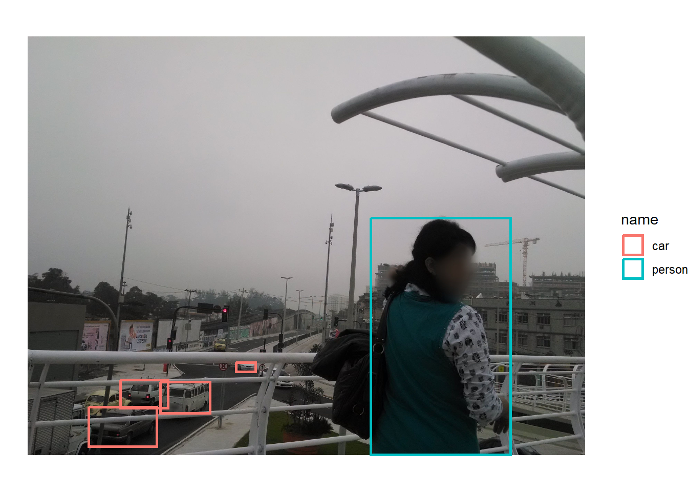
It should be relatively straightforward to count the number of cars and persons in this image
detections %>%
  group_by(name) %>%
  summarise(count = n())
# # A tibble: 2 × 2
#   name   count
#   <chr>  <int>
# 1 car        4
# 2 person     1
Exercise
- Repeat this for another random image in the data set.
- Write a function to repeat it for 10 images and display the number of cars, persons and bikes in each image.
- The code as it is written is very brittle and does not account for incorrect outputs, invalid conversions etc. Modify the function to intelligently catch the errors and gracefully fail.
- Display the number cars and persons in each image in the entire dataset, based on the location of the image.
Conclusion
While computer vision offers promising applications for planning practice, it remains a tool with significant limitations that planners must carefully consider before implementation. It is crucial to recognize that these techniques frequently struggle with accuracy in real-world conditions—misclassifying objects, failing to detect items in poor lighting or weather, and exhibiting biases based on their training data.
The technology’s tendency to produce confident-seeming results that mask underlying uncertainties can lead to flawed policy decisions if planners treat automated analyses as truth rather than imperfect interpretations requiring human validation. Moreover, computer vision systems often perform poorly on the nuanced, context-dependent assessments that planning work demands—such as evaluating neighborhood character, assessing building quality, or understanding the social dynamics of public spaces. Privacy concerns, high implementation costs, and the risk of perpetuating existing inequities through biased algorithms further complicate adoption. While computer vision may eventually become a valuable supplementary tool for certain planning tasks, it should be approached with healthy skepticism, robust validation processes, and clear understanding that human judgment, community input.
Nikhil Kaza
Professor
My research interests include urbanization patterns, local energy policy and equity