Matching Messy Texts
The Problems of Free Form Text
One of the joys of language is that there is an infinite variety of ways in which we can express ourselves. Conventions vary. People are likely to run afoul of grammatical and spelling conventions depending on their background, attention to detail and adherence to convention. This expressive variety becomes a disadvantage for a data analyst who wants to analyse text. Urban datasets frequently contain free form language; names, addresses, surveys, regulations, complaints, tweets, posts, newspaper reports, plans, interviews, ordinances etc. When the text is not standardised and restricted, they pose problems for a data analyst who is trying to reduce and distill the information, often ignoring the context and conventions that the gives meaning to the text. The text is then wrangled, standardised or ignored. In this blog, I will show how one might attempt to wrangle text. I also want to highlight the decisions that the analyst makes that severely distort the meaning and introduce errors.
All clean datasets are alike. But each messy dataset is messy in its own way — Prener paraphrasing Wickham paraprhasing Tolstoy
Data & Required Packages
The Worker Adjustment and Retraining Notification Act (WARN) requires employers with 100 or more employees (generally not counting those who have worked less than six months in the last 12 months and those who work an average of less than 20 hours a week) to provide at least 60 calendar days advance written notice of a plant closing and mass lay-off affecting 50 or more employees at a single site of employment. In Ohio, the Department of Job and Family Services is in charge of collecting and archiving the notices. Research by Cleveland Federal Reserve Bank suggests that these notices are useful bellwethers for economic conditions in the state. We are limiting our analysis to 2024 data for Ohio.
Historical data for WARN is at
- Krolikowski, Pawel M. and Kurt G. Lunsford. 2020. “Advance Layoff Notices and Labor Market Forecasting.” Federal Reserve Bank of Cleveland, Working Paper no. 20-03. https://doi.org/10.26509/frbc-wp-202003
In this blog, I am going to use another business listings dataset from Infogroup called ReferenceUSA to establish additional information about the business that is listed in the WARN database. ReferenceUSA data for the US can be obtained from UNC library. I obtained the WARN dataset from Ohio.
In this tutorial, I am going to use stringr, stringi, stringdist, postmastr, ellmer packages in addition to other packages in R.
library(tidyverse)
library(skimr)
library(readxl)

warn_df <-
  here("tutorials_datasets", "textmatching", "WARN_OH", "ohio_warn_2024.xlsm") %>%
  read_excel(sheet = "Sheet1")

names(warn_df)
# [1] "Firmname"
# [2] "Received_Date"
# [3] "Location"
# [4] "Affected_employees"
# [5] "Layoff_Date"
# [6] "Phone"
# [7] "Union: International of Bridge, Structural, Ornamental, Reinforcing Iron Workers, AFL-CIO, CLC"
# [8] "notice_ID"
# [9] "url"
Notice that there is no address field in the dataset. Sometimes the addresses are in the pdf documents that are downloaded from the url field. I am used the following code to download the pdfs and is provided for reference. The downloaded pdfs are [here]((https://www.dropbox.com/scl/fo/s5s8nfxmpqazivf37s5om/ACx9bwbp-z1qT1-InaAOC4w?rlkey=1flvs665dqhk8hisox8gtp0ur&st=c3uebuaa&dl=0)
user_agents <- c(
  "Mozilla/5.0 (Windows NT 10.0; Win64; x64) AppleWebKit/537.36 (KHTML, like Gecko) Chrome/58.0.3029.110 Safari/537.36",
  "Mozilla/5.0 (Macintosh; Intel Mac OS X 10_15_7) AppleWebKit/605.1.15 (KHTML, like Gecko) Version/14.0.3 Safari/605.1.15",
  "Mozilla/5.0 (Windows NT 10.0; WOW64; rv:54.0) Gecko/20100101 Firefox/54.0",
  "Mozilla/5.0 (X11; Ubuntu; Linux x86_64; rv:52.0) Gecko/20100101 Firefox/52.0",
  "Mozilla/5.0 (iPad; CPU OS 13_5 like Mac OS X) AppleWebKit/605.1.15 (KHTML, like Gecko) Version/13.1.1 Mobile/15E148 Safari/604.1"
)

for (i in 1:nrow(warn_df)){
  current_ua <- sample(user_agents, 1) # Using this to randomly sample user agents to avoid being blocked by servers.
  print(current_ua)
  tryCatch({
  download.file(URLencode(warn_df$url[i]),
                destfile = here("InputData", "pdfs", paste0(warn_df$notice_ID[i], ".pdf")),
                mode = 'wb',
                headers = c("User-Agent" = current_ua))
                Sys.sleep(.5)
  }, error = function(e) {print(paste("Error downloading file for notice_ID:", warn_df$notice_ID[i]))})
}
Using a LLM to Extract Addresses from PDFs
An entire post is dedicated to working with Large Language Models. I will not rehash much of it here. However, I will show how I used Claude Anthropic large language model to extract addresses from the pdfs. You will need to get an API key from Claude. You can adapt this code for other LLM relatively easily, but your results may vary.
library(ellmer)
library(jsonlite)

Sys.setenv("ANTHROPIC_API_KEY" = "YOUR_API_KEY_HERE")  # Replace with your actual API key

extraction_prompt <- function(file_name){paste0("
From the attached pdf document with filename ", file_name, ", only return the name of facility/firm and address of location where a firm/facility is closing. Extract the address in a single line format.
Ignore information about address for any other entity espectially government entities such as Office of Workforce Development or Rapid Response Unit or variations thereof. If you encounter address for that entity, skip it.
Ignore firms and addresses that are not in Ohio, OH.

Also extract whether bumping rights exist or not.
If the address or bumping rights information are not present in the text, return null for that field.
Return the result as a JSON list the contains JSON objects with three fields: 'facility_name' (string), 'address' (string) and 'bumping_rights' (true or false).
The output must be valid JSON that can be parsed by fromJSON() in R. Do not include any explanation or formatting outside the JSON.

Example output:
  {
    'facility_name': 'ABC Manufacturing',
    'address': '123 Main St, Springfield, OH 45501',
    'bumping_rights': true
    'file_name' : '000-24-002.pdf'
  }

Rules:
  - Only extract information that is clearly present
- Return null for missing information. Do not make up values
- Ensure valid JSON format
- No text outside the JSON response
- Multiple entries in JSON are allowed.
- No ``` blocks.


File Content:
<<PDF_FILE_CONTENT>>
 "
)}


pdf_paths <- here("tutorials_datasets", "text_matching", "WARN_OH", "pdfs") %>%
  list.files(full.names = T)

# For each file, create a prompt and content_pdf_file object

prompts_warn <- map(pdf_paths, function(f){
  list(extraction_prompt(content_pdf_file(f)@filename),
       content_pdf_file(f)
      )
})

claude_chat <- chat_anthropic(
  model = "claude-sonnet-4-5-20250929",  # Check to see what the name of the latest model is https://docs.claude.com/en/docs/about-claude/models/overview
  api_key = Sys.getenv("ANTHROPIC_API_KEY"), #
  system_prompt = "You are an expert at extracting structured information from unstructured text. Always return valid JSON.",
  params = list(max_tokens = 1000,temperature = 0.1)  # Low temperature for consistent extraction
)

chat_out <- parallel_chat_text(claude_chat,
                      prompts_warn
                      )
Parse the JSON output
The above is a very time consuming processes and produces a list of JSON strings. I have written it out as a text file here.
I am going to read them in and parse them as if I ran the Claude code. But of course, saving them to a disk distorted the file from a vector a string. So we need to do some processing to recover the vector of JSON strings.
First I am using readLines to read in the text file and collapse them into a single string.
chat_out2 <- here("tutorials_datasets", "textmatching", "WARN_OH", "claude_warn_extraction_responses.txt") %>%
  readLines() %>%
  paste(collapse = "\n")

chat_out2
# [1] "```json\n[\n {\n \"facility_name\": \"GDI Services (Amazon Warehouse)\",\n \"address\": \"1550 W Main St, West Jefferson, OH 43162\",\n \"bumping_rights\": false,\n \"file_name\": \"000-24-002.pdf\"\n },\n {\n \"facility_name\": \"GDI Services (Amazon Warehouse)\",\n \"address\": \"1245 Beech Rd SW, New Albany, OH 43054\",\n \"bumping_rights\": false,\n \"file_name\": \"000-24-002.pdf\"\n },\n {\n \"facility_name\": \"GDI Services (Amazon Warehouse)\",\n \"address\": \"27400 Crossroads PKWY, Rossford, OH 43460\",\n \"bumping_rights\": false,\n \"file_name\": \"000-24-002.pdf\"\n }\n]\n```\n```json\n[\n {\n \"facility_name\": \"Lost Boys Interactive, LLC\",\n \"address\": \"Akron, Ohio\",\n \"bumping_rights\": false,\n \"file_name\": \"000-24-006.pdf\"\n },\n {\n \"facility_name\": \"Lost Boys Interactive, LLC\",\n \"address\": \"Columbus, Ohio\",\n \"bumping_rights\": false,\n \"file_name\": \"000-24-006.pdf\"\n },\n {\n \"facility_name\": \"Lost Boys Interactive, LLC\",\n \"address\": \"Lima, Ohio\",\n \"bumping_rights\": false,\n \"file_name\": \"000-24-006.pdf\"\n },\n {\n \"facility_name\": \"Lost Boys Interactive, LLC\",\n \"address\": \"North Royalton, Ohio\",\n \"bumping_rights\": false,\n \"file_name\": \"000-24-006.pdf\"\n },\n {\n \"facility_name\": \"Lost Boys Interactive, LLC\",\n \"address\": \"South Bloomfield, Ohio\",\n \"bumping_rights\": false,\n \"file_name\": \"000-24-006.pdf\"\n },\n {\n \"facility_name\": \"Lost Boys Interactive, LLC\",\n \"address\": \"Troy, Ohio\",\n \"bumping_rights\": false,\n \"file_name\": \"000-24-006.pdf\"\n },\n {\n \"facility_name\": \"Lost Boys Interactive, LLC\",\n \"address\": \"Upper Arlington, Ohio\",\n \"bumping_rights\": false,\n \"file_name\": \"000-24-006.pdf\"\n }\n]\n```\n```json\n[\n {\n \"facility_name\": \"Cygnus Home Service, LLC, d/b/a Yelloh\",\n \"address\": \"61000 Leyshom Drive, Byesville, OH 43723\",\n \"bumping_rights\": false,\n \"file_name\": \"000-24-075.pdf\"\n },\n {\n \"facility_name\": \"Cygnus Home Service, LLC, d/b/a Yelloh\",\n \"address\": \"1341 Freese Works Place, Galion, OH 44833\",\n \"bumping_rights\": false,\n \"file_name\": \"000-24-075.pdf\"\n },\n {\n \"facility_name\": \"Cygnus Home Service, LLC, d/b/a Yelloh\",\n \"address\": \"675 Wales Drive, Hartville, OH 44632\",\n \"bumping_rights\": false,\n \"file_name\": \"000-24-075.pdf\"\n },\n {\n \"facility_name\": \"Cygnus Home Service, LLC, d/b/a Yelloh\",\n \"address\": \"212 Hobart Drive, Hillsboro, OH 45133\",\n \"bumping_rights\": false,\n \"file_name\": \"000-24-075.pdf\"\n },\n {\n \"facility_name\": \"Cygnus Home Service, LLC, d/b/a Yelloh\",\n \"address\": \"2545 St. Johns Road, Lima, OH 45804\",\n \"bumping_rights\": false,\n \"file_name\": \"000-24-075.pdf\"\n },\n {\n \"facility_name\": \"Cygnus Home Service, LLC, d/b/a Yelloh\",\n \"address\": \"635 Independence Drive, Napolean, OH 43545\",\n \"bumping_rights\": false,\n \"file_name\": \"000-24-075.pdf\"\n },\n {\n \"facility_name\": \"Cygnus Home Service, LLC, d/b/a Yelloh\",\n \"address\": \"322 Arco Drive, Toledo, OH 43607\",\n \"bumping_rights\": false,\n \"file_name\": \"000-24-075.pdf\"\n },\n {\n \"facility_name\": \"Cygnus Home Service, LLC, d/b/a Yelloh\",\n \"address\": \"2991 S. County Road 25A, Troy, OH 45373\",\n \"bumping_rights\": false,\n \"file_name\": \"000-24-075.pdf\"\n }\n]\n```\n```json\n[\n {\n \"facility_name\": \"Vimo, Inc. dba GetInsured\",\n \"address\": null,\n \"bumping_rights\": false,\n \"file_name\": \"000-24-095.pdf\"\n },\n {\n \"facility_name\": \"D&A Consulting Services, dba GetInsured\",\n \"address\": null,\n \"bumping_rights\": false,\n \"file_name\": \"000-24-095.pdf\"\n }\n]\n```\n```json\n[\n {\n \"facility_name\": \"Nursery Supplies, Inc.\",\n \"address\": \"3175 Gilchrist Road, Mogadore, Ohio 44260\",\n \"bumping_rights\": false,\n \"file_name\": \"002-24-045.pdf\"\n }\n]\n```\n```json\n[\n {\n \"facility_name\": \"Epiroc Industrial Tools and Attachments LLC\",\n \"address\": \"820 Glaser Pkwy, Akron, OH 44306\",\n \"bumping_rights\": false,\n \"file_name\": \"002-24-058.pdf\"\n }\n]\n```\n```json\n[\n {\n \"facility_name\": \"Universal Screen Arts, Inc.\",\n \"address\": \"5581 Hudson Industrial Parkway, Hudson, OH 44236\",\n \"bumping_rights\": false,\n \"file_name\": \"002-24-072.pdf\"\n },\n {\n \"facility_name\": \"Universal Screen Arts, Inc.\",\n \"address\": \"6279 Hudson Crossing Parkway, Suite 100, Hudson, OH 44236\",\n \"bumping_rights\": false,\n \"file_name\": \"002-24-072.pdf\"\n }\n]\n```\n```json\n[\n {\n \"facility_name\": \"Nestlé USA, Inc.\",\n \"address\": \"5750 Harper Road, Solon, OH 44139\",\n \"bumping_rights\": false,\n \"file_name\": \"003-24-008.pdf\"\n },\n {\n \"facility_name\": \"Nestlé USA, Inc.\",\n \"address\": \"30003 Bainbridge Rd, Solon, OH 44139\",\n \"bumping_rights\": false,\n \"file_name\": \"003-24-008.pdf\"\n },\n {\n \"facility_name\": \"Nestlé USA, Inc.\",\n \"address\": \"30000 Bainbridge Road, Solon, OH 44139\",\n \"bumping_rights\": false,\n \"file_name\": \"003-24-008.pdf\"\n }\n]\n```\n```json\n[\n {\n \"facility_name\": \"ZIN Technologies, Inc.\",\n \"address\": \"6749 Engle Road, Middleburg Heights, OH 44130\",\n \"bumping_rights\": false,\n \"file_name\": \"003-24-009.pdf\"\n },\n {\n \"facility_name\": \"ZIN Technologies, Inc.\",\n \"address\": \"6745 Engle Road, Middleburg Heights, OH 44130\",\n \"bumping_rights\": false,\n \"file_name\": \"003-24-009.pdf\"\n }\n]\n```\n```json\n[\n {\n \"facility_name\": \"Metro Décor LLC\",\n \"address\": \"30320 Emerald Valley Parkway, Glenwillow, Ohio 44139\",\n \"bumping_rights\": false,\n \"file_name\": \"003-24-015.pdf\"\n },\n {\n \"facility_name\": \"Metro Décor LLC\",\n \"address\": \"28625 Fountain Parkway, Solon, Ohio 44139\",\n \"bumping_rights\": false,\n \"file_name\": \"003-24-015.pdf\"\n }\n]\n```\n```json\n[\n {\n \"facility_name\": \"CLE 2 Amazon\",\n \"address\": \"21500 Emery Rd, North Randall, OH 44128\",\n \"bumping_rights\": false,\n \"file_name\": \"003-24-023.pdf\"\n }\n]\n```\n```json\n[\n {\n \"facility_name\": \"Associated Materials, LLC\",\n \"address\": \"3773 State Road, Cuyahoga Falls, OH 44223\",\n \"bumping_rights\": false,\n \"file_name\": \"003-24-024.pdf\"\n }\n]\n```\n```json\n[\n {\n \"facility_name\": \"ProMedica Skilled Nursing and Rehabilitation at MetroHealth\",\n \"address\": \"4229 Pearl Road, Cleveland, OH 44109\",\n \"bumping_rights\": false,\n \"file_name\": \"003-24-028.pdf\"\n }\n]\n```\n```json\n[\n {\n \"facility_name\": \"Xellia Pharmaceuticals USA LLC\",\n \"address\": \"200 Northfield Rd., Bedford, OH 44146\",\n \"bumping_rights\": null,\n \"file_name\": \"003-24-048.pdf\"\n }\n]\n```\n```json\n[\n {\n \"facility_name\": \"Aramark Facility Services, LLC at Cleveland Browns Stadium\",\n \"address\": \"100 Alfred Lerner Way, Cleveland, OH\",\n \"bumping_rights\": false,\n \"file_name\": \"003-24-055.pdf\"\n }\n]\n```\n```json\n[\n {\n \"facility_name\": \"Airgas USA, LLC\",\n \"address\": \"6055 Rockside Woods Blvd North, Independence, OH 44131\",\n \"bumping_rights\": false,\n \"file_name\": \"003-24-067.pdf\"\n }\n]\n```\n```json\n[\n {\n \"facility_name\": \"Swissport USA, Inc.\",\n \"address\": \"5300 Riverside Dr, Cleveland, OH 44135\",\n \"bumping_rights\": false,\n \"file_name\": \"003-24-070.pdf\"\n }\n]\n```\n```json\n[\n {\n \"facility_name\": \"True Value Company, L.L.C.\",\n \"address\": \"26025 First Street, Westlake, OH 44145-1400\",\n \"bumping_rights\": null,\n \"file_name\": \"003-24-082.pdf\"\n }\n]\n```\n```json\n[\n {\n \"facility_name\": \"American Sugar Refining, Inc.\",\n \"address\": \"2075 E 65th St., Cleveland, OH 44103\",\n \"bumping_rights\": null,\n \"file_name\": \"003-24-088.pdf\"\n }\n]\n```\n```json\n[\n {\n \"facility_name\": \"First Student\",\n \"address\": \"42242 Albrecht Road, Elyria, OH 44035\",\n \"bumping_rights\": null,\n \"file_name\": \"004-24-021.pdf\"\n }\n]\n```\n```json\n[\n {\n \"facility_name\": \"Inservco Inc. d/b/a Vexos\",\n \"address\": \"110 Commerce Drive, LaGrange, OH 44050\",\n \"bumping_rights\": false,\n \"file_name\": \"004-24-057.pdf\"\n }\n]\n```\n```json\n[\n {\n \"facility_name\": \"Nordson Corporation\",\n \"address\": \"555 Jackson Street, Amherst, OH 44001\",\n \"bumping_rights\": true,\n \"file_name\": \"004-24-079.pdf\"\n },\n {\n \"facility_name\": \"Nordson Corporation\",\n \"address\": \"444 Gordon Ave, Amherst, OH 44001\",\n \"bumping_rights\": true,\n \"file_name\": \"004-24-079.pdf\"\n },\n {\n \"facility_name\": \"Nordson Corporation\",\n \"address\": \"200 Nordson Drive, Amherst, OH 44001\",\n \"bumping_rights\": true,\n \"file_name\": \"004-24-079.pdf\"\n },\n {\n \"facility_name\": \"Nordson Corporation\",\n \"address\": \"100 Nordson Drive, Amherst, OH 44001\",\n \"bumping_rights\": true,\n \"file_name\": \"004-24-079.pdf\"\n }\n]\n```\n```json\n[\n {\n \"facility_name\": \"Libra Industries, LLC\",\n \"address\": \"7770 Division Drive, Mentor, Ohio 44060\",\n \"bumping_rights\": false,\n \"file_name\": \"005-24-074.pdf\"\n }\n]\n```\n```json\n[\n {\n \"facility_name\": \"Libra Industries, LLC\",\n \"address\": \"7770 Division Drive, Mentor, Ohio 44060\",\n \"bumping_rights\": false,\n \"file_name\": \"005-24-091.pdf\"\n }\n]\n```\n```json\n[\n {\n \"facility_name\": \"Anheuser-Busch\",\n \"address\": \"1611 Marietta Ave SE, Canton, OH 44707\",\n \"bumping_rights\": false,\n \"file_name\": \"006-24-061.pdf\"\n }\n]\n```\n```json\n[\n {\n \"facility_name\": \"PPC Flexible Packaging LLC\",\n \"address\": \"9465 Edison St NE, Alliance, OH 44601\",\n \"bumping_rights\": false,\n \"file_name\": \"006-24-084.pdf\"\n }\n]\n```\n```json\n[\n {\n \"facility_name\": \"Newell Brands Distribution LLC\",\n \"address\": \"175 Heritage Drive, Pataskala, OH 43062\",\n \"bumping_rights\": false,\n \"file_name\": \"007-24-003.pdf\"\n }\n]\n```\n```json\n[\n {\n \"facility_name\": \"Marsden Services, L.L.C.\",\n \"address\": \"11999 National Rd SW Etna, OH 43018\",\n \"bumping_rights\": false,\n \"file_name\": \"007-24-004.pdf\"\n }\n]\n```\n```json\n[\n {\n \"facility_name\": \"VS Direct Fulfillment, LLC\",\n \"address\": \"5959 Bigger Road, Kettering, OH 45440\",\n \"bumping_rights\": false,\n \"file_name\": \"007-24-005.pdf\"\n }\n]\n```\n```json\n[\n {\n \"facility_name\": \"Linamar Structures USA (Michigan) Inc.\",\n \"address\": \"507 W Indiana St, Edon, OH 43518\",\n \"bumping_rights\": false,\n \"file_name\": \"007-24-010.pdf\"\n }\n]\n```\n```json\n[\n {\n \"facility_name\": \"SAVOR at Nutter Center\",\n \"address\": \"3640 Colonel Glenn Highway, Fairborn, OH 45324\",\n \"bumping_rights\": null,\n \"file_name\": \"007-24-014.pdf\"\n }\n]\n```\n```json\n[\n {\n \"facility_name\": \"IAC Wauseon, LLC\",\n \"address\": \"555 W. Linfoot Street, Wauseon, OH 43567\",\n \"bumping_rights\": true,\n \"file_name\": \"007-24-018.pdf\"\n }\n]\n```\n```json\n[\n {\n \"facility_name\": \"Amsive, LLC\",\n \"address\": \"3303 West Tech Road, Miamisburg, Ohio 45342\",\n \"bumping_rights\": false,\n \"file_name\": \"007-24-022.pdf\"\n }\n]\n```\n```json\n[\n {\n \"facility_name\": \"Honeywell Intelligrated LLC\",\n \"address\": \"475 E. High Street, London, OH 43140\",\n \"bumping_rights\": false,\n \"file_name\": \"007-24-030.pdf\"\n }\n]\n```\n```json\n[\n {\n \"facility_name\": \"Bon Appetit Management Co.\",\n \"address\": \"100 Smith Lane, Granville, OH\",\n \"bumping_rights\": false,\n \"file_name\": \"007-24-033.pdf\"\n }\n]\n```\n```json\n[\n {\n \"facility_name\": \"Insight Direct USA, Inc.\",\n \"address\": \"8337 Green Meadows Drive N, Lewis Center, OH 43035\",\n \"bumping_rights\": false,\n \"file_name\": \"007-24-035.pdf\"\n }\n]\n```\n```json\n[\n {\n \"facility_name\": \"RK Industries, Inc\",\n \"address\": \"725 N Locust St, Ottawa, OH 45875\",\n \"bumping_rights\": false,\n \"file_name\": \"007-24-042.pdf\"\n }\n]\n```\n```json\n[\n {\n \"facility_name\": \"Cygnus Home Service, LLC, d/b/a Yelloh\",\n \"address\": \"675 Wales Drive, Hartville, OH 44632\",\n \"bumping_rights\": false,\n \"file_name\": \"007-24-044.pdf\"\n },\n {\n \"facility_name\": \"Cygnus Home Service, LLC, d/b/a Yelloh\",\n \"address\": \"212 Hobart Drive, Hillsboro, OH 45133\",\n \"bumping_rights\": false,\n \"file_name\": \"007-24-044.pdf\"\n },\n {\n \"facility_name\": \"Cygnus Home Service, LLC, d/b/a Yelloh\",\n \"address\": \"2254 Rice Road, Jackson, OH 45640\",\n \"bumping_rights\": false,\n \"file_name\": \"007-24-044.pdf\"\n }\n]\n```\n```json\n[\n {\n \"facility_name\": \"Delta Apparel, Inc.\",\n \"address\": \"102 Reliance Drive, Hebron, Ohio 43025\",\n \"bumping_rights\": false,\n \"file_name\": \"007-24-051.pdf\"\n }\n]\n```\n```json\n[\n {\n \"facility_name\": \"idX Corporation dba idX Dayton\",\n \"address\": \"2875 Needmore Road, Dayton, OH 45414\",\n \"bumping_rights\": false,\n \"file_name\": \"007-24-054.pdf\"\n }\n]\n```\n```json\n[\n {\n \"facility_name\": \"Global Medical Response\",\n \"address\": \"8261 State Route 235, Dayton, Ohio 45424\",\n \"bumping_rights\": false,\n \"file_name\": \"007-24-059.pdf\"\n },\n {\n \"facility_name\": \"Global Medical Response\",\n \"address\": \"106 Royan Street, Sidney, Ohio 45365\",\n \"bumping_rights\": false,\n \"file_name\": \"007-24-059.pdf\"\n }\n]\n```\n```json\n[\n {\n \"facility_name\": \"ZF Active Safety US Inc\",\n \"address\": \"1750 Production Drive, Findlay, OH 45840\",\n \"bumping_rights\": null,\n \"file_name\": \"007-24-066.pdf\"\n }\n]\n```\n```json\n[\n {\n \"facility_name\": \"Faurecia Exhaust Systems\",\n \"address\": \"1255 Archer Dr, Troy, OH 45373\",\n \"bumping_rights\": false,\n \"file_name\": \"007-24-068.pdf\"\n }\n]\n```\n```json\n[\n {\n \"facility_name\": \"IAC Wauseon, LLC\",\n \"address\": \"555 W. Linfoot Street, Wauseon, OH 43567\",\n \"bumping_rights\": true,\n \"file_name\": \"007-24-073.pdf\"\n }\n]\n```\n```json\n[\n {\n \"facility_name\": \"P. Graham Dunn, Inc.\",\n \"address\": \"630 Henry St., Dalton, OH 44618\",\n \"bumping_rights\": false,\n \"file_name\": \"007-24-077.pdf\"\n }\n]\n```\n```json\n[\n {\n \"facility_name\": \"idX Corporation dba idX Dayton\",\n \"address\": \"2875 Needmore Road, Dayton, OH 45414\",\n \"bumping_rights\": false,\n \"file_name\": \"007-24-089.pdf\"\n }\n]\n```\n```json\n[\n {\n \"facility_name\": \"American Freight Stores, LLC\",\n \"address\": \"109 Innovation Court, Delaware, OH 43015\",\n \"bumping_rights\": false,\n \"file_name\": \"007-24-090.pdf\"\n }\n]\n```\n```json\n[\n {\n \"facility_name\": \"Spartech LLC\",\n \"address\": \"925 W. Gasser Road, Paulding, OH, 45879\",\n \"bumping_rights\": false,\n \"file_name\": \"007-24-092.pdf\"\n }\n]\n```\n```json\n[\n {\n \"facility_name\": \"Decorative Panels International, Inc.\",\n \"address\": \"2900 Hill Avenue, Toledo, Ohio 43607\",\n \"bumping_rights\": false,\n \"file_name\": \"009-24-017.pdf\"\n }\n]\n```\n```json\n[\n {\n \"facility_name\": \"Optum\",\n \"address\": \"100 N Byrne Rd, Toledo, OH 43607\",\n \"bumping_rights\": false,\n \"file_name\": \"009-24-041.pdf\"\n }\n]\n```\n```json\n[\n {\n \"facility_name\": \"FCA US LLC - Toledo Assembly Complex\",\n \"address\": \"4400 Chrysler Drive, Toledo, OH 43608\",\n \"bumping_rights\": true,\n \"file_name\": \"009-24-085.pdf\"\n }\n]\n```\n```json\n[\n {\n \"facility_name\": \"Mobis North America LLC\",\n \"address\": \"3900 Stickney Ave., Toledo, Ohio 43608\",\n \"bumping_rights\": null,\n \"file_name\": \"009-24-086.pdf\"\n }\n]\n```\n```json\n[\n {\n \"facility_name\": \"KUKA Toledo Production Operations, LLC\",\n \"address\": \"3770 Stickney Ave, Toledo, OH 43608\",\n \"bumping_rights\": true,\n \"file_name\": \"009-24-087.pdf\"\n }\n]\n```\n```json\n[\n {\n \"facility_name\": \"Walmart\",\n \"address\": \"3579 S High St, Columbus, OH 43207\",\n \"bumping_rights\": false,\n \"file_name\": \"011-24-011.pdf\"\n }\n]\n```\n```json\n[\n {\n \"facility_name\": \"Genpact LLC\",\n \"address\": \"7000 Cardinal Place, Dublin, OH 43017\",\n \"bumping_rights\": false,\n \"file_name\": \"011-24-012.pdf\"\n }\n]\n```\n```json\n[\n {\n \"facility_name\": \"BrightView Enterprise Solutions, LLC\",\n \"address\": \"6530 W. Campus Oval #300, New Albany, OH 43054\",\n \"bumping_rights\": false,\n \"file_name\": \"011-24-019.pdf\"\n }\n]\n```\n```json\n[\n {\n \"facility_name\": \"Sid Tool Co., Inc. dba MSC Industrial Direct Co., Inc.\",\n \"address\": \"1568 Georgesville Rd., Columbus, Ohio\",\n \"bumping_rights\": false,\n \"file_name\": \"011-24-020.pdf\"\n }\n]\n```\n```json\n[\n {\n \"facility_name\": \"EVO Transportation & Energy Services, Inc.\",\n \"address\": \"3115 E. 17th Avenue, Columbus, OH 43219\",\n \"bumping_rights\": false,\n \"file_name\": \"011-24-031.pdf\"\n }\n]\n```\n```json\n[\n {\n \"facility_name\": \"Express, LLC and Express Fashion Operations, LLC\",\n \"address\": \"1 Express Drive, Columbus, OH 43230\",\n \"bumping_rights\": false,\n \"file_name\": \"011-24-032.pdf\"\n },\n {\n \"facility_name\": \"Express, LLC and Express Fashion Operations, LLC\",\n \"address\": \"235 North 4th Street, Columbus, OH 43215\",\n \"bumping_rights\": false,\n \"file_name\": \"011-24-032.pdf\"\n }\n]\n```\n```json\n[\n {\n \"facility_name\": \"Arlington Contact Lens Service, Inc.\",\n \"address\": \"2250 International St. Columbus, OH 43228\",\n \"bumping_rights\": false,\n \"file_name\": \"011-24-034.pdf\"\n }\n]\n```\n```json\n[\n {\n \"facility_name\": \"Bath & Body Works Logistics Services, LLC\",\n \"address\": \"1 Limited Parkway, Columbus, OH 43230\",\n \"bumping_rights\": false,\n \"file_name\": \"011-24-036.pdf\"\n }\n]\n```\n```json\n[\n {\n \"facility_name\": \"Djafi Trucking Company, LLC\",\n \"address\": \"2491 East Dublin Granville Road, Columbus, OH 43229\",\n \"bumping_rights\": false,\n \"file_name\": \"011-24-037.pdf\"\n }\n]\n```\n```json\n[\n {\n \"facility_name\": \"Sodexo, Inc and Affiliates\",\n \"address\": \"4892 BLAZER PKWY, Dublin, OH 43017\",\n \"bumping_rights\": null,\n \"file_name\": \"011-24-038.pdf\"\n }\n]\n```\n```json\n[\n {\n \"facility_name\": \"Charter Communications Customer Contact Center\",\n \"address\": \"1600 Dublin Road, Columbus, OH 43215\",\n \"bumping_rights\": false,\n \"file_name\": \"011-24-047.pdf\"\n }\n]\n```\n```json\n[\n {\n \"facility_name\": \"Bath & Body Works Logistics Services, LLC\",\n \"address\": \"1 Limited Parkway, Columbus, OH 43230\",\n \"bumping_rights\": false,\n \"file_name\": \"011-24-049.pdf\"\n }\n]\n```\n```json\n[\n {\n \"facility_name\": \"Pitney Bowes Inc.\",\n \"address\": \"6111 Bixby Road, Canal Winchester, OH\",\n \"bumping_rights\": false,\n \"file_name\": \"011-24-053.pdf\"\n }\n]\n```\n```json\n[\n {\n \"facility_name\": \"Pitney Bowes Inc. Global Ecommerce facility\",\n \"address\": \"6111 Bixby Road, Canal Winchester, OH\",\n \"bumping_rights\": null,\n \"file_name\": \"011-24-060.pdf\"\n }\n]\n```\n```json\n[\n {\n \"facility_name\": \"DHL Supply Chain\",\n \"address\": \"6200 Winchester Blvd, Canal Winchester, OH 43110\",\n \"bumping_rights\": false,\n \"file_name\": \"011-24-080.pdf\"\n }\n]\n```\n```json\n[\n {\n \"facility_name\": \"Centerpoint Health\",\n \"address\": \"3420 Atrium Blvd., Suite 102, Franklin, OH 45005\",\n \"bumping_rights\": null,\n \"file_name\": \"012-24-007.pdf\"\n }\n]\n```\n```json\n[\n {\n \"facility_name\": \"St. Bernard Soap Company\",\n \"address\": \"5177 Spring Grove Avenue, Cincinnati, OH 45217\",\n \"bumping_rights\": true,\n \"file_name\": \"013-24-001.pdf\"\n }\n]\n```\n```json\n[\n {\n \"facility_name\": \"Oak View Group\",\n \"address\": \"525 Elm St, Cincinnati, OH 45202\",\n \"bumping_rights\": false,\n \"file_name\": \"013-24-029.pdf\"\n }\n]\n```\n```json\n[\n {\n \"facility_name\": \"Mauser Packaging Solutions\",\n \"address\": \"8200 Broadwell Road, Cincinnati, OH 45244\",\n \"bumping_rights\": true,\n \"file_name\": \"013-24-039.pdf\"\n }\n]\n```\n```json\n[\n {\n \"facility_name\": \"Barclays Services, LLC\",\n \"address\": \"1435 Vine St, Cincinnati, OH 45202\",\n \"bumping_rights\": false,\n \"file_name\": \"013-24-043.pdf\"\n }\n]\n```\n```json\n[\n {\n \"facility_name\": \"Nordic Consulting Group, Inc.\",\n \"address\": \"1701 Mercy Health Place, Cincinnati, OH 45237\",\n \"bumping_rights\": null,\n \"file_name\": \"013-24-050.pdf\"\n }\n]\n```\n```json\n[\n {\n \"facility_name\": \"Pepsi Beverages Company Cincinnati\",\n \"address\": \"2121 Sunnybrook Dr, Cincinnati, OH 45237\",\n \"bumping_rights\": true,\n \"file_name\": \"013-24-083.pdf\"\n }\n]\n```\n```json\n[\n {\n \"facility_name\": \"Northside Regional Medical Center\",\n \"address\": \"500 Gypsy Lane, Youngstown, OH 44501\",\n \"bumping_rights\": false,\n \"file_name\": \"017-24-062.pdf\"\n }\n]\n```\n```json\n[\n {\n \"facility_name\": \"Hillside Rehabilitation Hospital\",\n \"address\": \"8747 Squires Lane NE, Warren, OH 44484\",\n \"bumping_rights\": false,\n \"file_name\": \"018-24-063.pdf\"\n }\n]\n```\n```json\n[\n {\n \"facility_name\": \"Hillside Rehabilitation Hospital\",\n \"address\": \"8747 Squires Lane NE Warren, OH 44484\",\n \"bumping_rights\": false,\n \"file_name\": \"018-24-064.pdf\"\n }\n]\n```\n```json\n[\n {\n \"facility_name\": \"Trumbull Regional Medical Center\",\n \"address\": \"1350 E. Market Street, Warren, OH 44483\",\n \"bumping_rights\": false,\n \"file_name\": \"018-24-065.pdf\"\n }\n]\n```\n```json\n[\n {\n \"facility_name\": \"Mohawk Fine Papers, Inc.\",\n \"address\": \"6800 Center Road, Ashtabula, OH 44004\",\n \"bumping_rights\": false,\n \"file_name\": \"019-24-016.pdf\"\n }\n]\n```\n```json\n[\n {\n \"facility_name\": \"General Aluminum, LLC\",\n \"address\": \"1370 Chamberlain Blvd. Conneaut, Ohio 44030\",\n \"bumping_rights\": false,\n \"file_name\": \"019-24-081.pdf\"\n }\n]\n```\n```json\n[\n {\n \"facility_name\": \"Commercial Vehicle Group (CVG) Chillicothe\",\n \"address\": \"75 Chamber Dr., Chillicothe, OH 45601\",\n \"bumping_rights\": false,\n \"file_name\": \"020-24-013.pdf\"\n }\n]\n```\n```json\n[\n {\n \"facility_name\": \"Post Consumer Brands\",\n \"address\": \"3775 Lancaster New Lexington Rd. SE, Lancaster, OH 43130\",\n \"bumping_rights\": true,\n \"file_name\": \"020-24-056.pdf\"\n }\n]\n```\n```json\n[\n {\n \"facility_name\": \"American Freight Stores, LLC\",\n \"address\": \"109 Innovation Court, Delaware, OH 43015\",\n \"bumping_rights\": false,\n \"file_name\": \"077-24-093.pdf\"\n }\n]\n```\n```json\n[]\n```\n```json\n[\n {\n \"facility_name\": \"Family Dollar\",\n \"address\": \"780 S3 W PLANE ST, BETHEL, Clermont, OH 45106-1313\",\n \"bumping_rights\": null,\n \"file_name\": \"999-24-026.pdf\"\n },\n {\n \"facility_name\": \"Family Dollar\",\n \"address\": \"1300 7990 READING RD, CINCINNATI, Hamilton, OH 45237-2112\",\n \"bumping_rights\": null,\n \"file_name\": \"999-24-026.pdf\"\n },\n {\n \"facility_name\": \"Family Dollar\",\n \"address\": \"3549 6704 N RIDGE RD, MADISON, Lake, OH 44057-2639\",\n \"bumping_rights\": null,\n \"file_name\": \"999-24-026.pdf\"\n },\n {\n \"facility_name\": \"Family Dollar\",\n \"address\": \"3967 1121 N REYNOLDS RD, TOLEDO, Lucas, OH 43615-4755\",\n \"bumping_rights\": null,\n \"file_name\": \"999-24-026.pdf\"\n },\n {\n \"facility_name\": \"Family Dollar\",\n \"address\": \"4052 650 N UNIVERSITY BLVD, MIDDLETOWN, Butler, OH 45042-3356\",\n \"bumping_rights\": null,\n \"file_name\": \"999-24-026.pdf\"\n },\n {\n \"facility_name\": \"Family Dollar\",\n \"address\": \"4674 5527 BRIDGETOWN RD, Cincinnati, Hamilton, OH 45248-4329\",\n \"bumping_rights\": null,\n \"file_name\": \"999-24-026.pdf\"\n },\n {\n \"facility_name\": \"Family Dollar\",\n \"address\": \"4936 511 S BREIEL BLVD, MIDDLETOWN, Butler, OH 45044-5111\",\n \"bumping_rights\": null,\n \"file_name\": \"999-24-026.pdf\"\n },\n {\n \"facility_name\": \"Family Dollar\",\n \"address\": \"5778 9302 MILES AVENUE, CLEVELAND, Cuyahoga, OH 44105-6116\",\n \"bumping_rights\": null,\n \"file_name\": \"999-24-026.pdf\"\n },\n {\n \"facility_name\": \"Family Dollar\",\n \"address\": \"5819 440 N JAMES H MCGEE BLVD, DAYTON, Montgomery, OH 45402-6531\",\n \"bumping_rights\": null,\n \"file_name\": \"999-24-026.pdf\"\n },\n {\n \"facility_name\": \"Family Dollar\",\n \"address\": \"5948 519 S 2ND ST, RIPLEY, Brown, OH 45167-1307\",\n \"bumping_rights\": null,\n \"file_name\": \"999-24-026.pdf\"\n },\n {\n \"facility_name\": \"Family Dollar\",\n \"address\": \"6226 2372 CLEVELAND AVE, COLUMBUS, Franklin, OH 43211-1610\",\n \"bumping_rights\": null,\n \"file_name\": \"999-24-026.pdf\"\n },\n {\n \"facility_name\": \"Family Dollar\",\n \"address\": \"6364 1250 E 105TH ST, CLEVELAND, Cuyahoga, OH 44108-3568\",\n \"bumping_rights\": null,\n \"file_name\": \"999-24-026.pdf\"\n },\n {\n \"facility_name\": \"Family Dollar\",\n \"address\": \"6925 3577 E Livingston Avenue, Columbus, Franklin, OH 43227-2235\",\n \"bumping_rights\": null,\n \"file_name\": \"999-24-026.pdf\"\n },\n {\n \"facility_name\": \"Family\n```json\n[\n {\n \"facility_name\": \"Volta Charging Industries, LLC\",\n \"address\": null,\n \"bumping_rights\": false,\n \"file_name\": \"999-24-027.pdf\"\n }\n]\n```\n```json\n[\n {\n \"facility_name\": null,\n \"address\": null,\n \"bumping_rights\": false,\n \"file_name\": \"999-24-040.pdf\"\n }\n]\n```\n```json\n[\n {\n \"facility_name\": \"Lost Boys Interactive, LLC\",\n \"address\": \"Akron, Ohio\",\n \"bumping_rights\": false,\n \"file_name\": \"999-24-071.pdf\"\n },\n {\n \"facility_name\": \"Lost Boys Interactive, LLC\",\n \"address\": \"Columbus, Ohio\",\n \"bumping_rights\": false,\n \"file_name\": \"999-24-071.pdf\"\n },\n {\n \"facility_name\": \"Lost Boys Interactive, LLC\",\n \"address\": \"lima, Ohio\",\n \"bumping_rights\": false,\n \"file_name\": \"999-24-071.pdf\"\n },\n {\n \"facility_name\": \"Lost Boys Interactive, LLC\",\n \"address\": \"North Royalton, Ohio\",\n \"bumping_rights\": false,\n \"file_name\": \"999-24-071.pdf\"\n },\n {\n \"facility_name\": \"Lost Boys Interactive, LLC\",\n \"address\": \"South Bloomfield, Ohio\",\n \"bumping_rights\": false,\n \"file_name\": \"999-24-071.pdf\"\n },\n {\n \"facility_name\": \"Lost Boys Interactive, LLC\",\n \"address\": \"Troy, Ohio\",\n \"bumping_rights\": false,\n \"file_name\": \"999-24-071.pdf\"\n },\n {\n \"facility_name\": \"Lost Boys Interactive, LLC\",\n \"address\": \"Upper Arlington, Ohio\",\n \"bumping_rights\": false,\n \"file_name\": \"999-24-071.pdf\"\n }\n]\n```\n```json\n[\n {\n \"facility_name\": \"kaleo, Inc.\",\n \"address\": null,\n \"bumping_rights\": false,\n \"file_name\": \"999-24-076.pdf\"\n }\n]\n```\n```json\n[\n {\n \"facility_name\": null,\n \"address\": null,\n \"bumping_rights\": false,\n \"file_name\": \"999-24-078.pdf\"\n }\n]\n```"
Extract individual JSON objects from the text. We are going to use Regular Expressions to search and extract.
# The pattern uses DOTALL (?s) to allow '.' to match newlines,
# and a non-greedy capture group (.*?) to grab only the content
# between the code fences.
json_regex <- "(?s)```json\n(.*?)\n```"

# str_match_all finds all matches and returns a list of matrices.
# The JSON content is in the second column of the matrix.
extracted_matches <- str_match_all(chat_out2, json_regex)[[1]]

# Extract the second column (Capture Group 1: the raw JSON string)
json_blocks_vector <- extracted_matches[, 2]
Explanation of the Regular Expression
Here is a breakdown of its components:
-
“(?s)": This is an inline flag (modifier) that enables the DOTALL (or single-line) mode for the entire regular expression. In this mode, the dot (.) metacharacter matches any single character, including newline characters (\n). By default, the dot usually excludes newlines.
-
“```json\n”: This part matches the literal string “```json” followed by a newline character.
-
(.*?):
-"(” and “)": These parentheses create a capturing group, which saves the matched text for later use.
- “.” : In combination with the (?s) flag, this matches any single character, including newlines.
- “*?": This is a non-greedy (or lazy) quantifier, meaning it matches zero or more occurrences of the preceding element (.) but as few times as possible to allow the rest of the pattern to match. It stops as soon as it encounters the pattern that follows it. -"\n```": This matches a literal newline character followed by “```”, which serves as the end boundary for the non-greedy match.
In summary, this regex looks for the first occurrence of “```json” followed by a newline, and then lazily captures all the content after it until it finds the next newline character. It is likely used to extract a single line of data (which might contain spaces) that follows a “json” header in a multi-line string.
It might helpful to see what this regex does on a sample text. In this example the second JSON is malformed in the sample text with no closing code fence “```”
# Sample text with multiple lines
text <- "Some introductory text.
Here is a block of data:

```json
{\"key\": \"value\", \"count\": 123}

````
```json
[1, 2, 3]
End of data block

"
str_match_all(text, json_regex)
# [[1]]
#      [,1]
# [1,] "```json\n{\"key\": \"value\", \"count\": 123}\n\n```"
#      [,2]
# [1,] "{\"key\": \"value\", \"count\": 123}\n"
Exercise
- The above is necessary only to extract JSON strings from a larger text. Adapt the code to work on the output of the LLM.
The following code cleans up the extracted JSON strings. It removes the code fences and ensures that the JSON objects are complete by appending necessary closing brackets if they are missing.
json_blocks_vector <- json_blocks_vector[str_detect(json_blocks_vector, "\\{")]  # Keep only responses that contain JSON objects

library(jsonlite)

warn_extracted_df <-
  map(json_blocks_vector, function(x){
  tryCatch({
    fromJSON(x, simplifyDataFrame = TRUE, flatten = TRUE)
  }, error = function(e){
    tibble(facility_name = NA_character_,
           address = NA_character_,
           bumping_rights = NA,
           file_name = NA_character_)
  })
  }) %>%
  bind_rows()

warn_extracted_df %>% glimpse()
# Rows: 123
# Columns: 4
# $ facility_name  <chr> "GDI Services (Amazon Warehouse)", "GDI Services (Amazo…
# $ address        <chr> "1550 W Main St, West Jefferson, OH 43162", "1245 Beech…
# $ bumping_rights <lgl> FALSE, FALSE, FALSE, FALSE, FALSE, FALSE, FALSE, FALSE,…
# $ file_name      <chr> "000-24-002.pdf", "000-24-002.pdf", "000-24-002.pdf", "…


warn_df <-
  warn_extracted_df %>%
  mutate(notice_ID = str_remove(file_name, "\\.pdf$")) %>%
  filter(!is.na(address)) %>%
  left_join(warn_df, by = c("notice_ID" = "notice_ID"))


warn_df %>% glimpse()
# Rows: 120
# Columns: 13
# $ facility_name                                                                                    <chr> …
# $ address                                                                                          <chr> …
# $ bumping_rights                                                                                   <lgl> …
# $ file_name                                                                                        <chr> …
# $ notice_ID                                                                                        <chr> …
# $ Firmname                                                                                         <chr> …
# $ Received_Date                                                                                    <chr> …
# $ Location                                                                                         <chr> …
# $ Affected_employees                                                                               <dbl> …
# $ Layoff_Date                                                                                      <chr> …
# $ Phone                                                                                            <chr> …
# $ `Union: International of Bridge, Structural, Ornamental, Reinforcing Iron Workers, AFL-CIO, CLC` <chr> …
# $ url                                                                                              <chr> …
Parsing the Addresses
Most geocoders expect an address that is properly standardised (e.g. South - S, Bvld - Boulevard ) and spelling errors corrected. This is important as user entered text about addresses rely on personal and local convention rather than standardisation. We can use postmastr to standardise and parse addresses.
postmastr is not yet available on CRAN, but can be installed from github using
remotes::install_github("slu-openGIS/postmastr")
postmastr works by following the precise sequence of the following steps.
Preparation
First there is a need to create a unique ID for unique addresses, so that only unique addresses are parsed. A quick look at the address column reveals that it has newlines \n in some of the entries. Let’s replace it with a space.
In the following code, I am replacing all the diacritics, e.g.ř, ü, é, è by transliterating to Latin alphabet. This is not strictly necessary but is useful to remember that some place names are in Spanish in the US. Some databases store the diacritics and some don’t. Apologies to speakers of other languages.
It is always a good idea to have one case. We are going to use the upper case.
warn_df <- warn_df %>%
        mutate(address = str_replace_all(address, "[[:space:]]", " "),
               address = stringi::stri_trans_general(address, "Latin-ASCII"),
               address = str_remove_all(address, "[[:punct:]]"),
               address = str_to_upper(address)

               )

warn_df$address %>% head()
# [1] "1550 W MAIN ST WEST JEFFERSON OH 43162"
# [2] "1245 BEECH RD SW NEW ALBANY OH 43054"
# [3] "27400 CROSSROADS PKWY ROSSFORD OH 43460"
# [4] "AKRON OHIO"
# [5] "COLUMBUS OHIO"
# [6] "LIMA OHIO"
library(postmastr)
warn_df <- pm_identify(warn_df, var = "address")
warn_min <- pm_prep(warn_df, var = "address", type ='street') # There do not seem to be any addresses that are based on intersections. So we are using the type=street.
nrow(warn_df)
# [1] 120
nrow(warn_min)
# [1] 101
You should notice the difference in the number of rows. 19 observations are dropped.
Extract Zipcodes and States
Zipcodes come in two formats. A 5 digit variety and 5-4 digit variety. pm_postal_parse is able to parse both types, though in this instance only 5 digit codes are present.
warn_min <- pm_postal_parse(warn_min)
In this instance only state present in the dataset is OH. First we need to create a dictonary in case OH is spelled out in different ways such as Ohio or OHIO. Fortunately, this dataset only contains OH. If not, use pm_append to add different instances of the state name to the dictionary.
ohDict <- pm_dictionary(locale = "us", type = "state", filter = "OH", case = "upper")
ohDict
# # A tibble: 2 × 2
#   state.output state.input
#   <chr>        <chr>
# 1 OH           OH
# 2 OH           OHIO

(warn_min <- pm_state_parse(warn_min, dict=ohDict))
# # A tibble: 101 × 4
#    pm.uid pm.address                     pm.state pm.zip
#     <int> <chr>                          <chr>    <chr>
#  1      1 1550 W MAIN ST WEST JEFFERSON  OH       43162
#  2      2 1245 BEECH RD SW NEW ALBANY    OH       43054
#  3      3 27400 CROSSROADS PKWY ROSSFORD OH       43460
#  4      4 AKRON                          OH       <NA>
#  5      5 COLUMBUS                       OH       <NA>
#  6      6 LIMA                           OH       <NA>
#  7      7 NORTH ROYALTON                 OH       <NA>
#  8      8 SOUTH BLOOMFIELD               OH       <NA>
#  9      9 TROY                           OH       <NA>
# 10     10 UPPER ARLINGTON                OH       <NA>
# # ℹ 91 more rows
ohCityDict <- pm_dictionary(locale = "us", type = "city", filter = "OH", case = "upper")
(warn_min <- pm_city_parse(warn_min, dictionary = ohCityDict))
# # A tibble: 101 × 5
#    pm.uid pm.address            pm.city          pm.state pm.zip
#     <int> <chr>                 <chr>            <chr>    <chr>
#  1      1 1550 W MAIN ST        WEST JEFFERSON   OH       43162
#  2      2 1245 BEECH RD SW      NEW ALBANY       OH       43054
#  3      3 27400 CROSSROADS PKWY ROSSFORD         OH       43460
#  4      4 <NA>                  AKRON            OH       <NA>
#  5      5 <NA>                  COLUMBUS         OH       <NA>
#  6      6 <NA>                  LIMA             OH       <NA>
#  7      7 <NA>                  NORTH ROYALTON   OH       <NA>
#  8      8 <NA>                  SOUTH BLOOMFIELD OH       <NA>
#  9      9 <NA>                  TROY             OH       <NA>
# 10     10 <NA>                  UPPER ARLINGTON  OH       <NA>
# # ℹ 91 more rows
Parsing Street, Numbers and Direction
We can use similar functions to parse out the street number.
warn_min <- warn_min %>%
             pm_house_parse()
Directionality of the street is little of a challenge. North could mean direction or a street name North St. Postmastr has logic already built into it to distinguish these two cases. By default, postmastr uses dic_us_dir dictionary.
dic_us_dir
# # A tibble: 20 × 2
#    dir.output dir.input
#    <chr>      <chr>
#  1 E          E
#  2 E          East
#  3 N          N
#  4 N          North
#  5 NE         NE
#  6 NE         Northeast
#  7 NE         North East
#  8 NW         NW
#  9 NW         Northwest
# 10 NW         North West
# 11 S          S
# 12 S          South
# 13 SE         SE
# 14 SE         Southeast
# 15 SE         South East
# 16 SW         SW
# 17 SW         Southwest
# 18 SW         South West
# 19 W          W
# 20 W          West
We have already converted our strings to upper cases rather than leaving it in the sentence case as dic_us_dir assumes. We will have to modify the dictionary to fit our useccase.
dic_us_dir <- dic_us_dir %>%
              mutate(dir.input = str_to_upper(dir.input))


warn_min <- warn_min %>%
             pm_streetDir_parse(dictionary = dic_us_dir) %>%
             pm_streetSuf_parse() %>%
             pm_street_parse(ordinal = TRUE, drop = TRUE)
Once we have parsed data, we add our parsed data back into the source.
warn_parsed <- pm_replace(warn_min, source = warn_df) %>%
               pm_rebuild(output="short", keep_parsed = 'yes')
Now that it is straightforward to geocode the addresses since they are all standardised.
Exercise
-
Use
tidygeocoderto see if the parsed addresses are geocoded correctly. Check for whether single line addresses can be geocoded correctly. How much improvement did you get? Was it worth the effort? -
Use
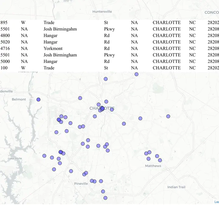
tmapto visualiase the locations of where the layoffs are occuring in Ohio.
Matching Names
Notice that in WARN data there are no NAICS codes, an industrial classification system that is commonly used (Other older classification is called SIC). So it is hard to tell which industry is being affected by these layoffs. Fortunately, another dataset has names and NAICS codes. So just as we matched parsed addresses to latitude an longitude, we can try and match names to NAICS codes. However, names are more idiosyncratic than addresses.
Here are some rules, I came up using iterative methods. They are not exhaustive nor are they representative of what you might want to with other datasets.
library(stringi)
library(stringr)
# I am trying to remove common words in the name that can impact string similarity scores. Add to the list or modify to suit.
removalwords <- c("CORP", "CORPORATION", "SERVICE", "SERVICES", "CO", "GROUP", "HOLDINGS", "MANAGEMENT", "LTD", "INC", "LLC", "L.L.C.", "PC", "PLLC", "SOLUTIONS", "COMPANY", "COMPANIES", "MANAGEMENT", "MGMNT", "USA", "US")
placenames <- tigris::places(state="OH", progress_bar = FALSE) %>% sf::st_set_geometry(NULL) %>% pull(NAME) %>% toupper()
compnames <- warn_parsed %>%
rename(company = facility_name) %>%
select(company, pm.zip) %>%
mutate(
orig_company = company,
company = str_squish(company), # Removes leading and trailing white spaces
company = str_remove_all(company, "\\&[A-Za-z]*;"), # This removes some HTML tags like " < etc.
company = str_remove_all(company, "\\t|\\n|\\r"), # This removes newlines and some other returns
company = str_remove_all(company, "[[:punct:]]"), # This removes punctuations marks such as `,`, `'`, '?
company = str_replace_all(company, "\\.", "\ "), # This replaces . with a space.
company = str_replace(company, "d/b/a ", "DBA"), #This replaces d/b/a with DBA
company = stringi::stri_trans_general(company, "Latin-ASCII"), # substitute unicode characters such as é, ü, ñ etc.
company = str_to_upper(company), # Convert to upper case.
company = str_remove_all(company, paste0("\\b(",paste0(removalwords, collapse="|"), ")\\b")), # Remove all the words that are in the list above.
company = str_remove_all(company, paste0("\\b(",paste0(placenames, collapse="|"), ")\\b")), # Remove place names from the company names. This may not work out well if the company is called for e.g. Cleveland Plastics.
name1 = str_split(company, "DBA", n=2, simplify = T)[,1] %>% str_squish(), #The following two lines split the names of the company at DBA (Doing Business As).
name2 = str_split(company, "DBA", n=2, simplify = T)[,2] %>% str_squish()
)
We can make educated guesses about what the NAICS codes for the WARN dataset are going to by searching for some common substrings associated with the industry. For example, sector 72 is Accommodation and Food Services.
compnames <- compnames %>%
  mutate(NAICS2 = case_when(
    str_detect(company, "\\bMEDICAl\\b") ~ "62",
    str_detect(company, '\\bAIRLINES\\b') ~ "48",
    str_detect(company, '\\bRESTAURANT|RSTRNT\\b') ~ "72",
    str_detect(company, '\\bCAFE|BAR\\b') ~ "72",
    str_detect(company, "\\bFITNESS\\b") ~ "71",
    str_detect(company, "\\bHOTEL|MOTEL|INN\\b") ~ "72",
    str_detect(company, "\\bHOSPITAL\\b") ~ "62",
    str_detect(company, "\\bSCHOOL|UNIVERSITY|COLLEGE|ACADEMY\\b") ~ "61",
    str_detect(company, "\\bGROCERY|SUPERMARKET|MARKET\\b") ~ "44",
    str_detect(company, "\\bFACTORY|MANUFACTURING|MFG|PLANT|INDUSTRIES|INDUSTRIAL\\b") ~ "31",
    str_detect(company, "\\bCONSTRUCTION|CONTRACTORS|CONSTR\\b") ~ "23",
    str_detect(company, "\\bTRANSPORTATION|TRANSIT|LOGISTICS|FREIGHT|TRUCKING|HAULING\\b") ~ "48",
    str_detect(company, "\\bRETAIL|STORE|STORES|SHOPPING\\b") ~ "44",
    str_detect(company, "\\bTECHNOLOGY|TECH|SOFTWARE|INFORMATICS|INFORMATION SYSTEMS|INTERACTIVE\\b") ~ "51",
    TRUE ~ NA_character_

  )
  )
We still need to find out the NAICS code for 90 companies.
Fuzzy String Matching
For the rest of the dataset, we are going to use Reference USA dataset that has names and NAICS codes.
refUSA <- here("tutorials_datasets", "textmatching", "WARN_OH",  "ohio_business_2022.csv") %>% read_csv() %>%
  mutate(orig_company = company,
         company = str_to_upper(company),
         company = str_remove_all(company, "[[:punct:]]"),
         company = str_replace_all(company, "\\.", "\ "),
         company = str_remove_all(company, paste0("\\b(",paste0(removalwords,  collapse="|"), ")\\b")),
         company = str_squish(company)
  ) %>%
  mutate(NAICS2 = str_sub(naics_code, start=1, end=2)) %>%
  filter(company != "")
Exercise
- Try matching (exact) on names from the WARN dataset to the RefUSA dataset. What is the match rate?
You will notice that the match rate is on exact match is not great because of various spellings and typos. Thus asking the question what is the row that matches the company name string in RefUSA dataset. So we instead ask a different question. How similar are two strings? To do that we have to understand the notion of distance between two strings. There are number of such distances. Here are some common ones.
- Levenshtein distance (lv) the minimum number of single-character edits (insertions, deletions or substitutions) required to change one word into the other
- Damerau–Levenshtein (dl) distance is the minimum number of operations (consisting of insertions, deletions or substitutions of a single character, or transposition of two adjacent characters) required to change one word into the other.
- Optimal String Alignment (osa) uses Damerau–Levenshtein distance but each substring may only be edited once.
- Hamming distance (hamming) is the number of positions with same symbol/character in both strings of equal length.
- Longest common substring distance (lcs) is the minimum number of symbols/characters that need to be removed to make the two strings the same.
- Jaro-winker distance (jw) is a distance that is derived from the lengths of two strings, number of shared symbols an their transpositions.
- soundex is distance between two strings when they are translated to phonetic code.
These are by no means exhaustive. They can even be improved upon (e.g. weighting spelling errors based on keyboard layouts.)
In the following code, I am going to use a bunch of different string distance algorithms, find the most similar string based on each algorithm and pick the string that is selected by many different algorithms.
library(stringdist)

distance_methods<-c('osa', 'dl','lcs','jw', 'soundex')

# While loops are terrible in R it is easy to program them. Better for readability.

for (i in 1:dim(compnames)[1]){
  # Only focus on the subset of data that we did not already hard code the NAICS
  if(is.na(compnames$NAICS2[i])){
    company <- compnames[i,]
    name1 <- company$name1
    name2 <- company$name2
    zcta <- company$pm.zip

    # Create a target dataset.
    refusa_select <- refUSA %>% filter(zipcode == zcta)

    # The following creates a vector of potential candidates (best match based on different algorithms)
    # In the following, I am using similarity score of 0.75 or higher. Adjust this for tighter or looser matches.

    closestmatch <-
      map_int(distance_methods,  # for each distance method
              possibly(
                function(x){
                  name1sim <- stringsim(name1, refusa_select$company, method= x) # Create a string similarity between name1 and refusa name
                  name2sim <- stringsim(name2, refusa_select$company, method=x)  # Create a string similarity between name2 and refusa name
                  # Apply a threshold
                  name1sim <- ifelse(name1sim<0.75, NA, name1sim)
                  name2sim <- ifelse(name2sim<0.75, NA, name2sim)
                  # Between name1sim an name2sim, pick the one with the highest score.
                  k <- pmax(name1sim, name2sim, na.rm=T) %>% which.max()
                  return(ifelse(length(k)!=0,k,NA_integer_))
                },
                NA_integer_
              )
      ) %>%
      .[!is.na(.)]

    # Of the distance methods, only select the matches that pass the threshold and pick the NAICS code that has the highest frequency. Note that this code does not break ties.i.e. there may be multiple NAICS that potentially picked by multiple algorithms, but this code picks the one that is at the top (possibly ordered)


    compnames$NAICS2[i]<-
      ifelse(length(closestmatch)>0,
               refusa_select[closestmatch,] %>%
               group_by(NAICS2) %>%
               summarize(no = n()) %>%
               slice_max(no, n=1, with_ties = FALSE) %>% select(NAICS2) %>% unlist() %>% unname(),
             NA_character_
      )

    rm(name1,name2,zcta,closestmatch)
  }
}
Of the 120 we are able to determine the NAICS codes for 65 companies, a 54.17 % hit rate. This is not quite acceptable, but we will stop here since it is already too long.
Exercise
- Use a different set string distance algorithms, esp ones based on n-grams.
- Instead of selecting strings with maximum similarity, select top 5 similar strings and then pick the string that appears in most of these algorithms.
- What other preprocessing can be done to improve the hit rate?
- Spot check to see if the hits are accurate?
Conclusions
As you noticed, a lot of text/string manipulation relies on understanding the linguistic conventions and is an iterative processes. What works in one context may not work in another and you should be prepared to adapt. You will encounter edge cases much more frequently in this type of work, than other kinds of data munging operations. Nonetheless, it is a useful skill to have. In particular, it is useful get familiar with using Regular Expressions to search for patterns within strings. However, use it judiciously.
Additional Resources
- Silge, Julia, and David Robinson. 2020. Text Mining with R. Sebastapol, CA: O' Reilly. https://www.tidytextmining.com/.
Nikhil Kaza
Professor
My research interests include urbanization patterns, local energy policy and equity