Introduction

Land suitability analysis has a long tradition in planning. Ian McHarg at Penn, pioneered the method of overlaying transparencies about suitability criteria, which then got translated into GIS with the advent of computers. Suitability analysis has many uses in planning. It can be used, for example, for

• Retail site selection
• Determining best locations for future land use (such as residential, agriculture, commercial etc..)
• Ecological planning for protecting natural habitats
• Prioritising investments (such as flood protection)
• Post-Disaster housing relocation (see Christian Karmath’s MP report)

These analyses have a long tradition in planning. In fact, my former doctoral advisor, Lew Hopkins, wrote a paper in 1977, on this topic and is still considered a classic. Dick Klosterman’s Planning Support System, WhatIf?™ relies heavily on land suitability analysis.

In this tutorial, I give a contrived example of finding suitable site for locating a landfill using rasters. Every cell is treated as potential alternative site for the landfill and is given a score based on different criteria (such as distance to schools, population centers etc.). The trick is to figure out a right combination of these scores to order the cells (alternatives). The analytical techniques used are rather straightforward and rely on simple raster algebra. As we will see, the skill is about picking the right kinds of criteria and making appropriate judgments about how to evaluate alternatives with respect to the criteria. Subjectivity and analyst’s bias is omnipresent in these steps. In particular, it is also subject to all sorts of other theoretical problems that the insistence on quantification obfuscates.

Requirements

Many new packages are introduced in this analysis including units (to systematically think and capture units such as km^2), fasterize (fast rasterization) and others such as rasterVis, terra, sf and tidycensus.

The datasets are available here

Additional resources

I strongly recommend that you read through R spatial by Robert Hijmans, the author of the raster and terra packages. In addition, you can also check out the R-exercises tagged as geospatial.

Land Suitability for Locating a Landfill

There are no accepted conventions for identifying the appropriate locations of landfills. Locating one, is a contentious topic, as it is a Locally Unwanted Land Use (LULU). Furthermore, there are many regulatory agencies that are involved in regulating the landfill locations including the Environmental Protection Agency.

In this example, I am going to use 4 arbitrary criteria

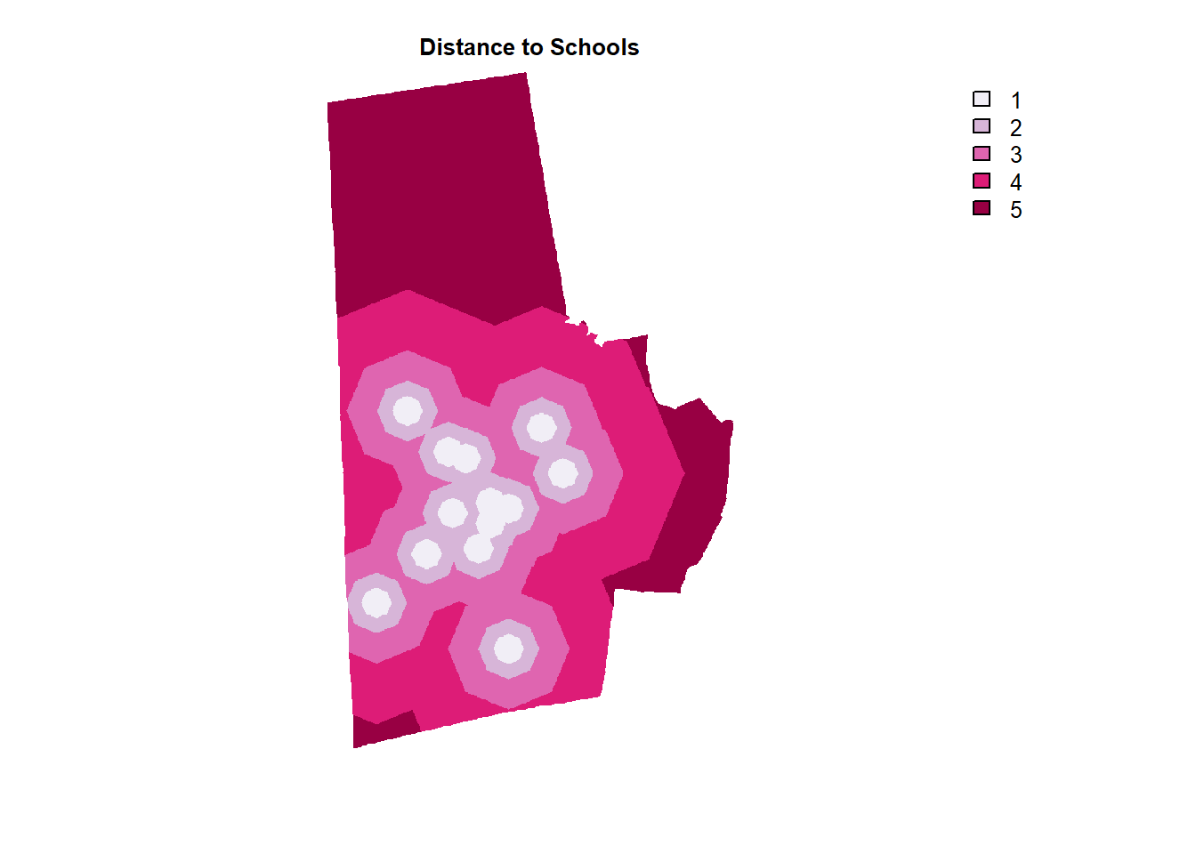
1. Distance to Schools. (Farther the better)
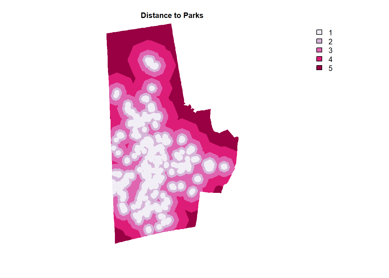
2. Distance to Parks. (Farther the better)
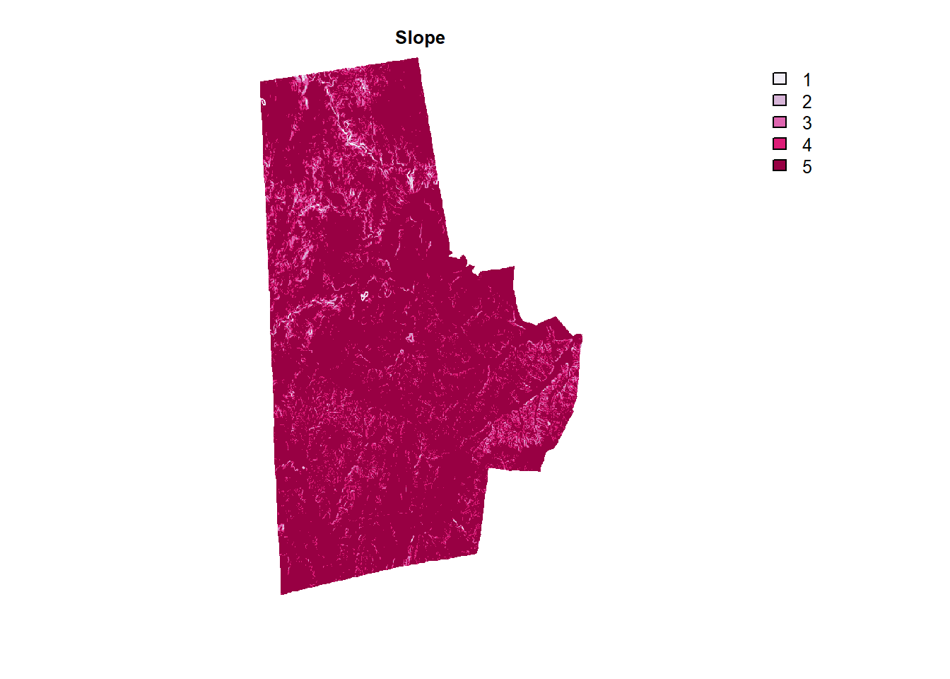
3. Slope (Flatter the better)
4. Distance to population centres (Sufficiently far, but no further)

But first set up the project crs by setting it to the crs of the land use raster and also create a template raster, by taking the extent and projection from a land use raster and setting every value to 0.

library(terra)
library(rasterVis)
library(here)
library(tidyverse)
library(fasterize)
library(sf)




lu_raster <- here("tutorials_datasets", "landsuitability", "c11_37063.img") %>% rast 
template_raster <- classify(lu_raster, cbind(0, 100, 0), right=FALSE) %>% raster::raster() #fasterize works with raster object instead of spatRaster object. Hence the conversion
project_crs <- crs(lu_raster)

vector_read_fn <- function(x){
      if(file.exists(x)){
          temp1 <- st_read(x, quiet=TRUE) %>% st_transform(project_crs)
          return(temp1)
      } 
}

Distance to Schools & Parks

The workhorse functions are gridDistance and classify both from the terra package.

gridDistance is a function that calculates the distance to cells of a SpatRaster when the path has to go through the centers of neighboring raster cells. This is effectively like buffering at multiple distances.

Xlassify is a function that (re)classifies groups of values to other values. For example, all values between 0 and 1000 become 1, and all values between 1000 and 2000 become 2 in the following code. In particular, see the rcl matrix argument in ?classify

schools <- here("tutorials_datasets", "landsuitability", "NCDurhamSchools", "SchoolPts.shp") %>% vector_read_fn()


schools_raster_dist <- schools %>% 
                  st_buffer(10) %>%  # Fasterize only works with polygons, so we create tiny buffers around the points
                  fasterize(raster= template_raster, background = 0) %>%
                  rast %>%  # Converting to SpRaster.
                  gridDistance(target=1) %>% # Check ?fasterize especially the `field argument on why target is 1.
                  mask(lu_raster) %>%
                  classify(rcl = matrix(c(0,1000,1, 1000,2000,2, 2000,4000,3, 4000,8000,4, 8000,Inf,5), ncol=3, byrow = T), include.lowest =T, right = F)

Similar approach can be taken to distance to parks. Here we have three different types of parks, including easement. We just select the geometry and treat them all the same. There is no need to buffer them, because they are already polygons.

parks <- here("tutorials_datasets", "landsuitability", "NCDurhamParksTrailsGreenways", "Parks.shp") %>% vector_read_fn() %>% dplyr::select(geometry)
future <- here("tutorials_datasets", "landsuitability", "NCDurhamParksTrailsGreenways", "Future_Parks.shp") %>% vector_read_fn() %>% dplyr::select(geometry)
easements <- here("tutorials_datasets", "landsuitability", "NCDurhamParksTrailsGreenways", "GreenwayEasementParcels.shp") %>% vector_read_fn() %>% dplyr::select(geometry)

parks_and_others <- reduce(list(parks, future, easements), rbind)
rm(parks, future, easements)



parks_others_raster_dist <- parks_and_others  %>% 
  fasterize(raster= template_raster, background =0) %>%
  rast() %>%
  gridDistance(target=1) %>%
  mask(lu_raster) %>%#Create a new Raster* object that has the same values as x, except for the cells that are NA (or other maskvalue) in a 'mask'.
  classify(rcl = matrix(c(0,500,1, 500,1000,2, 1000,2000,3, 2000,4000,4, 4000,Inf,5), ncol=3, byrow = T), include.lowest=T, right = FALSE)

Visualise them using the following code

library(RColorBrewer)
schools_raster_dist  %>% plot(col=brewer.pal(5, "PuRd"), type = "classes", axes=F, main = "Distance to Schools")

parks_others_raster_dist %>% plot(col=brewer.pal(5, "PuRd"), type = "classes", axes =F, main = "Distance to Parks")

Slope

Fortunately to calculate slopes in the US, there is an excellent package called elevatr that downloads the USGS Digital elevation model. USGS Digital elevation models (DEMs) are arrays of regularly spaced elevation values.

Once we acquire the raw elevation data, we can use the terrain function to create the slope raster.

Note the use of resample to make sure that the slope data that conforms to the extent, dimensions and resolution of the original land use dataset.

library(elevatr)
durham_slope <- get_elev_raster(template_raster, z = 11) %>% rast() %>%
                    terrain(v="slope", unit="degrees") %>%
                    resample(lu_raster, method= "bilinear") %>% 
                    mask(lu_raster) %>%
                    classify(rcl = matrix(c(0,5,5, 5,7,4, 7,10,3, 10,13,2, 13,Inf,1), ncol=3, byrow = T), include.lowest=T)

durham_slope  %>% plot(col=brewer.pal(5, "PuRd"), type = "classes", axes =F, main = "Slope")

More Complicated Distance Calculations

In this subsection, I am going to demonstrate how to use more complicated network distance calculations, instead of a geographic distance that we used earlier. We are going to use gdistance package by Jacob Van Etten. It is useful to peruse the vignette for the package. Remember raster can be treated as a network/graph that is mostly regular (except at the corners of the raster). Then the problem is simply finding the shortest route on the graph if the we can assign costs to the edges.

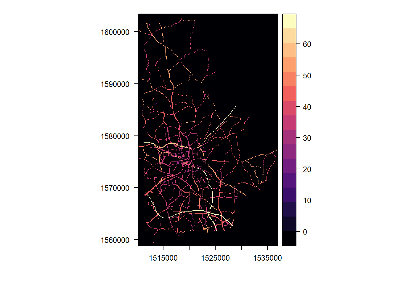
To do this, we take advantage of the highway network and its attributes. There is a SPEED_LMT, which we will treat as the speed to traverse that link. The LANES attribute can be used to construct the width of the road and then use it to construct the raster.

library(gdistance)

highways <- here("tutorials_datasets", "landsuitability", "Roads", "Roads.shp") %>% 
             vector_read_fn() %>% 
             filter(func_class != "Local Roads") %>%
             mutate(LANES = as.numeric(as.character(LANES)),
                     SPEED_LMT = as.numeric(as.character(SPEED_LMT)),
                    bufferwidth = ifelse(is.na(LANES), 30, LANES * 30/2)
                   )%>%
            st_buffer(dist = .$bufferwidth) %>% 
            fasterize(template_raster, field = "SPEED_LMT", fun='max')



highways[is.na(highways)] <- 0
levelplot(highways, margin = FALSE)

highways <- rast(highways)

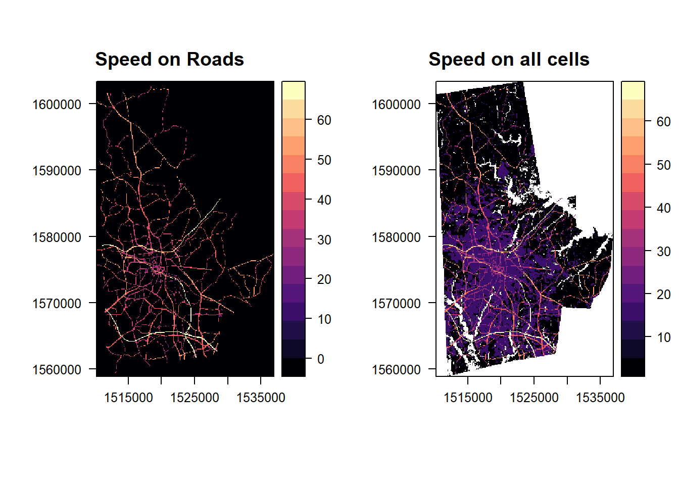
For the rest of the raster that are not covered by highways, we arbitarily assign a speed based on land cover class. In this instance, we assign of 15mph to developed cells and 5 mph to cells that are forests and other land covers. We also make water, wetlands impassable by assigning them NA speed. We take advantage of the fact that National Land Cover Dataset has two digit code, which the first digit representing a higher landuse type (Water, Developed etc.). Hence, the integer division by 10 using floor() discarding the remainder.

speed_raster <- floor(lu_raster / 10) %>%
                  classify(rcl = matrix(c(1,NA, 2,15, 3,5, 4,5, 5, 5, 6,5, 7,5, 8,5, 9, NA), ncol=2, byrow=T))
                    
                
combined_speed_raster <- max(speed_raster, highways)


p1 <- levelplot(raster(highways), margin = FALSE, main ='Speed on Roads')
p2 <- levelplot(raster(combined_speed_raster), margin=FALSE, main = "Speed on all cells")

library(gridExtra)
grid.arrange(p1,p2, ncol=2)

Exercise

• Feel free to experiment with other speeds based on other datasets.

In gdistance package, the edge weights on the neighbor graph are stored using a conductance framework (instead of a resistance) and the key concept is a transition matrix. It is stored as a sparse matrix. It is essentially captures which two cells are connected and how much conductance is there between the two cells. It is useful to work through some toy examples to understand how to construct the appropriate transition matrix.

Trmatx <- transition(1/(raster(combined_speed_raster)*0.44704) , function(x){1/mean(x)}, 8, symm=TRUE) %>%
          geoCorrection # 0.44704 is conversion between mph and m/s

Exercise

• This particular methodology assumes a number of things, including distances by traversing the cells is a good proxy for real travel distance. But sometimes, it may not be. For example, limited access highways can only accessed at very specific locations (interchanges). So least cost travel distance will have to account for the fact that sometimes you will have to travel futher to access a higher speed cell. How would you adjust this method to account for these features?

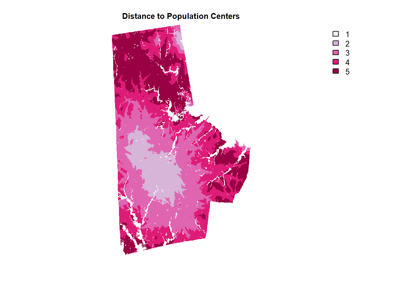
In this example, I am going to use population centres as defined high population density and high population and calculate the network distance to these centres for each pixel in the raster. I am arbitrarily setting that being 1200s is ideal and deviation in either direction is penalised. As usual, I am categorizing the distance raster.

library(units)
#library(tidycensus) # In Oct 2022, the census website was down.
#durham_blk <- get_decennial(geography = "block", variables = "P001001", state = "NC", county = "Durham", geometry = T, year = '2010') %>%
#                st_transform(crs=project_crs) %>% 
#                mutate(popdens = value/(st_area(.) %>% set_units(km^2)))


durham_blk <-  here("tutorials_datasets", "landsuitability", "Blocks", "2010_Census_Blocks.shp") %>% # This is all NC blocks
              st_read() %>%
              mutate(county_fips = str_sub(geoid10, start = 1L, end = 5L)) %>%
              filter(county_fips == "37063") %>% # Durham FIPS code
              st_transform(crs=project_crs) %>%
              mutate(popdens = total_pop/(st_area(.) %>% set_units(km^2)))
          
  

pop_concentrations <- durham_blk %>% 
                      filter(popdens>set_units(10000, 1/km^2) & total_pop > 300) %>% # Arbitrarily picking 10,000 people/km^2 and 300 people as thresholds
                      st_centroid()

dist_popcenters_raster <- accCost(Trmatx, pop_concentrations %>% as_Spatial()) %>% 
                              raster::calc(function(x){ceiling(5-(abs(x-1200)/300))}) %>%  # These are functions in raster not terra. Only using this because acCost gives raster not SpatRaster
                              raster::clamp(lower=1, upper=5, useValues=FALSE) %>% 
                              rast()

Exercise

• Convert output from accCost into a SpatRaster and use functions for terra to achieve the same result.

dist_popcenters_raster   %>% 
  mask(lu_raster) %>%
 plot(col=brewer.pal(5, "PuRd"), type = "classes", axes =F, main = "Distance to Population Centers")

Exercise

• Boolean (0-1/T-F) rasters have special meaning and arithmetic operations with boolean rasters are effectively boolean algebra. Sum of two boolean rasters is ‘OR’ and product of two boolean rasters is AND. Why?

• Use these features of Boolean rasters to effectively remove cells from consideration as alternatives to speed up processing. For example, a landfill may not be located on land that is already developed.

Multi-criteria Decision Making

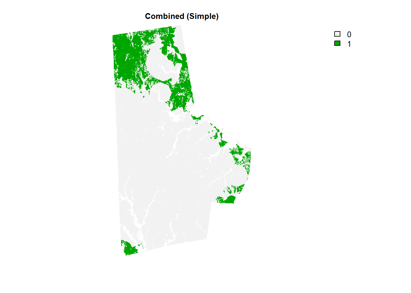
Until now, we have 4 criteria. Alternatives were assessed w.r.t. the criteria and there is forced consistency in the scales (1 is worst, 5 is best). Even though, these are ordinal scales, much of land suitability analyses treat them as numerical values. If so, then a simplest way is combine (add) them all and pick the best cells that score the highest (or at least above a threshold). See for example.

durham_stack <- c(schools_raster_dist, parks_others_raster_dist,durham_slope,dist_popcenters_raster)

combo_raster <- durham_stack[[1]] + durham_stack[[2]] + durham_stack[[3]] + durham_stack[[4]]

(combo_raster > 18)   %>% plot(type = "classes", axes =F, main = "Combined (Simple)")

Weighted Linear Combination

The above method treats every criteria equally. There is no reason to think that this should always be the case. If we assign weight to each of the four criteria and combine them according to those weights, then we are peforming weighted linear combination

combo_raster <-  durham_stack[[1]]*.2 + durham_stack[[2]]*.25 + durham_stack[[3]] * .4 + durham_stack[[4]]*.15  # Note the abitrary assignment of weights
(combo_raster > 4.9) %>% plot(type = "classes", axes =F, main = "Combined (Weighted)")  #Note the arbitrary cutoff

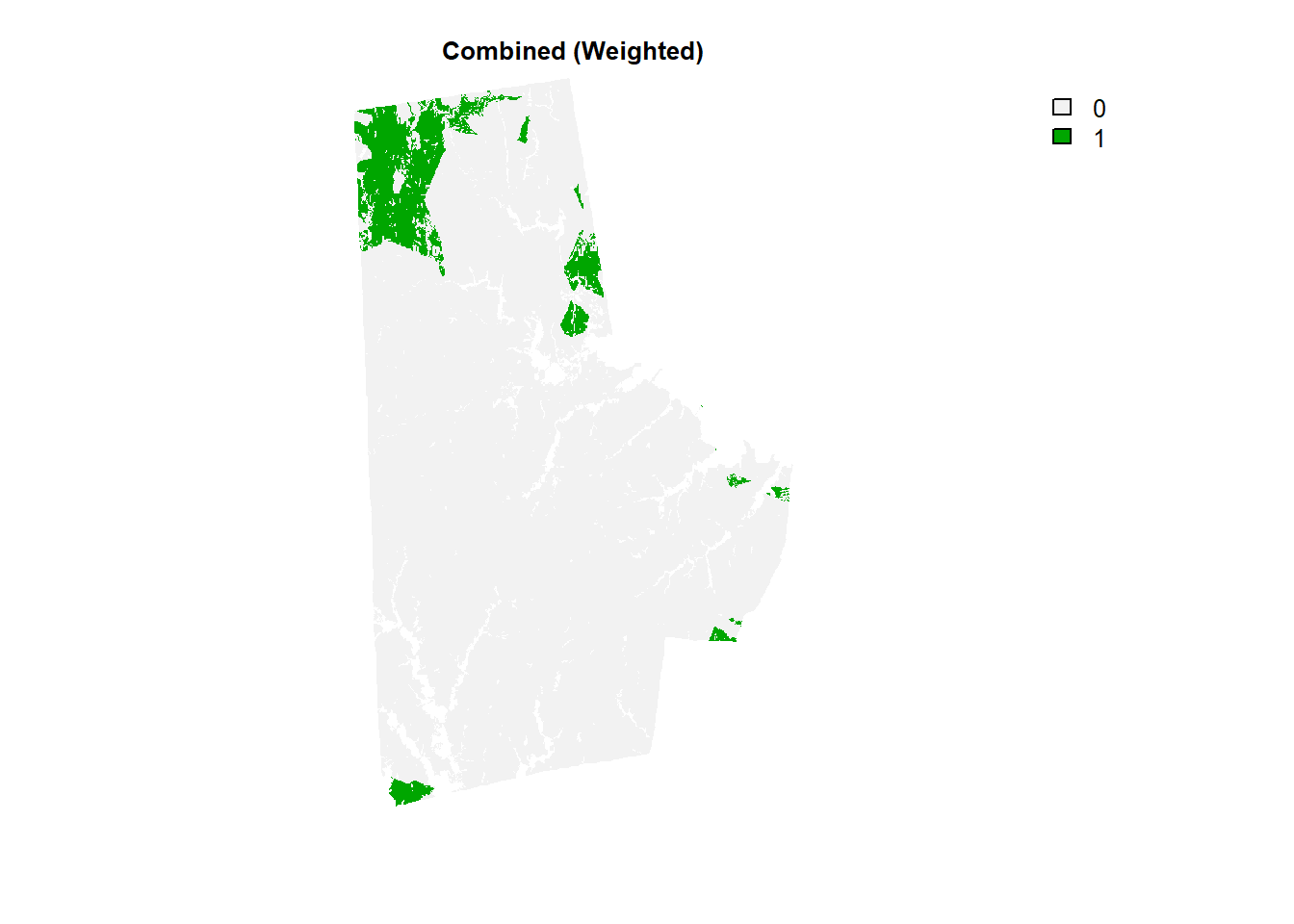
Note that the weights summing to 1 is a matter of convention, not a mathematical necessity (Sort of. It is a necessity, if you want to stick to 1-5 range.). More importantly, this arbitrary assignment of weights obscures judgments made by the analysts. That is distance from schools is half as important as slope (0.2 vs 0.4) and is 80% important as distance from parks etc. Furthermore, this weight assignment preserves consistency (i.e. transitive property). Distance to schools is 80% as important as distance to parks; distance to parks is 62.5% as important as slope and distance to school is (0.2/0.25) * (0.25/0.4) = 0.5 as important as slope.

**Exercise **

• Would it be better to eliminate the alternatives using boolean raster after WLC or before? If before, what is the appropriate step? Why? (Hint: Remember the difference between NA and 0).

Categorical Combination Method

While it is true that ordinal scales are treated as numeric often, they can also be treated as nominal by ignoring the order.

combo_raster <- 
 lapp(durham_stack, 
         fun = function(x){paste0(x[[1]],x[[2]],x[[3]],x[[4]], collapse="")}
         )

I am not displaying the raster because of enormous number of categories. 6 categories (5 levels + NA) in each raster layer with 4 layers, so the total number of combinations are 6^4 = 1,296. Clearly this is not reasonable number of categories from an analytical perspective and only few categories are going to be relevant, such as “5555” or “5455” etc. In such an instance it is probably better to reclassify ahead of time to sort for the relevant categories of interest (say for example 2) and restrict the total number of combinations (2^4=16).

Analytical Hierarchy Process

Developed by Thomas Satay in the 1970s, the Analytical Hierarchy Process (AHP) reduces the complexity of decisions by making the analyst only compare among two alternatives at a time, without sacrificing consistency. It has been widely used in decision making in different sectors (including hiring processes, environmental analyses, product development etc.). In the case of land suitability the AHP is useful to create a set of consistent weights and then applying the weighted linear combination method.

For a worked out example, please refer to this wikipedia article.

The key feature of AHP is the ranking among two criteria using a 1-9 scale, with 1 being the two criteria (e.g. A & B) being equally important and 9 being that A is extremely important compared to B. The rest of them are in between. The idea is to construct a matrix, whose elements represent a pairwise comparison. Also if A is extremely important compared to B (value = 9) the B to A comparison receives a reciprocal value (1/9). In this case, we have 4 criteria, (schools, parks, slope, population centres). By this logic, the diagonal elements are always 1.

AHPmatrix <- matrix(1,nrow=nlyr(durham_stack), ncol=nlyr(durham_stack))
row.names(AHPmatrix) <- colnames(AHPmatrix) <- c('Schools', 'Parks', "Slope", "PopulationCenters")
AHPmatrix[upper.tri(AHPmatrix)] <- c(2,5,3,4,7,2)

for(i in 1:dim(AHPmatrix)[1]){
  for(j in i:dim(AHPmatrix)[2])
    AHPmatrix[j,i] = 1/AHPmatrix[i,j]
}

Check to make sure that the AHP is indeed of the format required by the process. Once it is correct, the weights on the criteria are given by normalising the largest eigen vector of the matrix. But first we need to check the consistency of the matrix (i.e if the transitive property mostly holds). To do that we compute, \(CI := \frac{(\lambda_{max} - n)}{(n-1)}\) where \(\lambda_{max}\) is the largest eigen value of the matrix and \(n\) is the number of criteria.

CI <- (Mod(eigen(AHPmatrix)$values[1]) - 4)/3 #Using Modulus to ignore the zero imaginary part of the complex number.

The CI is compared to Random Consistency Index (RCI) from the table below. Pick the right RCI for the right number of criteria.

If Consistency Ration (CR) = CI/RCI < 0.10 is TRUE, then the AHP matrix is said to be consistent. If not, revise the weights till consistency is achieved.

Once consistency is achieved, the weights on the criteria are calculated by normalising the largest eigen vector of the matrix.

(weights <- eigen(AHPmatrix, symmetric =F)$vectors[,1] / sum(eigen(AHPmatrix, symmetric =F)$vectors[,1]))
# [1] 0.47975196+0i 0.33842037+0i 0.11097265+0i 0.07085501+0i

This demonstrates that Schools weigthed the highest followed by Parks in the pairwise weighting. The analysis then proceeds just like Weighted Linear Combination method.

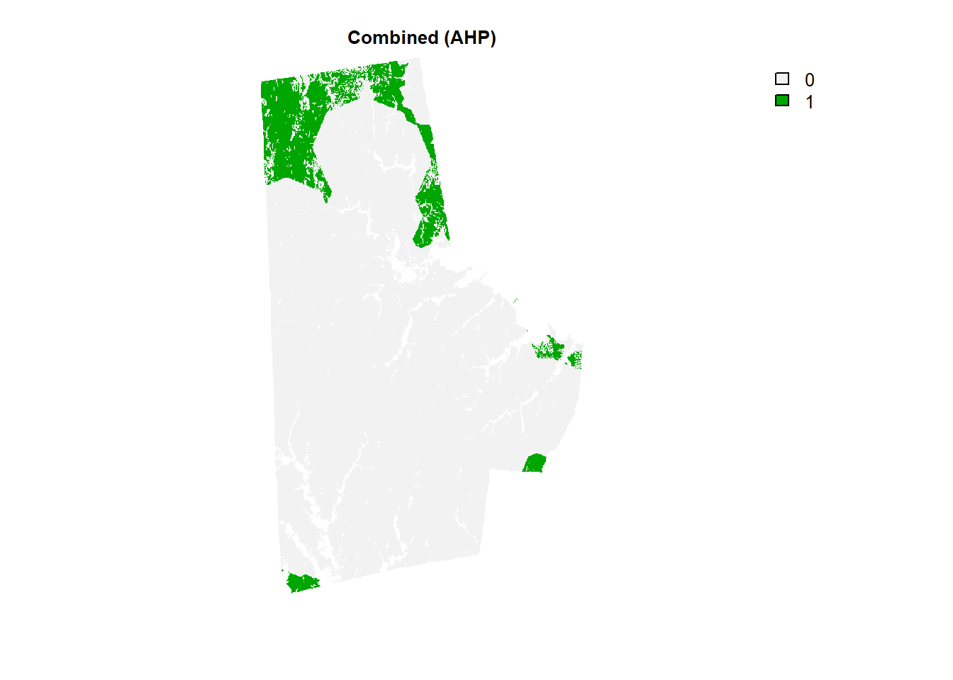
combo_raster <- durham_stack[[1]]*Re(weights)[1] + durham_stack[[2]]*Re(weights)[2] + durham_stack[[3]]*Re(weights)[3] + durham_stack[[4]]*Re(weights)[4]
                   
(combo_raster > 4.9) %>% plot(type = "classes", axes =F, main = "Combined (AHP)")

Exercise

• Experiment with increasing and decreasing the number of criteria.
• Experiment with different AHP matrices to identify consistency issues.

Conclusion

These are but some very basic and tried and tested methods used in planning practise. There are significant advances since the 70s including using fuzzy arithmetic, non-linear combinations etc. However, the point of many of these methods is not to identify the right locations, but provide a basis for discussion with relevant participants in the decision making processes.

It should however be noted that Multi-Criteria Decision Making and land suitability analyses are often presented as rational methods for making decisions about land uses. I hope I have demonstrated, in this tutorial, the subjective nature of the process. Please re-read the caveats.The things we choose to care about, says a lot about the values of the analyst.