Introduction to R & Rmarkdown
Getting started with R & Rmarkdown

Preliminaries
To get started with this course, you will need R. I strongly recommend Rstudio. To function correctly, RStudio needs R and therefore both need to be installed on your computer. If you already have these installed, please see this page to make sure you have up to date versions of the software. We will talk about other required software as we proceed further.
Why R?
- Great for reproducibility
- Great for statistics
- Great for data analysis and visualization
- Interdisciplinary & Extensible
- Open source & Cross Platform
- Most GIS operations can be done in R
See R-ecology for more details.
Actually, I see it as part of my job to inflict R on people who are perfectly happy to have never heard of it. Happiness doesn’t equal proficient and efficient. In some cases the proficiency of a person serves a greater good than their momentary happiness. – Patrick Burns: R-help (April 2005)
Why not Python? Or Julia? Or C++?
Mostly because I don’t know them well/or at all. They are probably great, but R works for me, for the most part. See Sebastian’s post on Why Python?.
Good Practices
- Keep track of who wrote what code at the top of the file and its purpose.
- Use comments liberally using “#”.
- Avoid
setwd()and use only relative paths. - Always use R projects
- Distinct components of the code should ideally be separate and be accessed using
source(). This improves legibility. - Use a consistent style within your code. For example, name all data frames to something ending in _df.
- Keep all of your source files for a project in the same directory, then use relative paths as necessary to access them.
- Memory is a problem for R, because it stores all objects in memory (mostly true). Follow good practice of deleting objects that you don’t need using
rm(). It is rarely necessary for you to use garbage collectiongc(). If you are running to into problems constantly- Consider upgrading RAM (It is becoming cheaper by the day).
- Consider if you can break up the data set and independently process them and reassemble them.
- Find alternative libraries and methods.
Basic R
Once you have R & Rstudio installed, run the following to see if it is working correctly.
1 + 1   #add 1 + 1
# [1] 2
a <- 2:5  #Assign vector 2:5 to a variable a
a      #print a to console
# [1] 2 3 4 5
runif(5)   #Generate 5 random numbers
# [1] 0.08783858 0.60768902 0.46983531 0.21926932 0.99419249
sessionInfo()     #What is my computer environment? (Mac, Windows, packages etc.)
# R version 4.4.1 (2024-06-14)
# Platform: aarch64-apple-darwin20
# Running under: macOS 15.6
#
# Matrix products: default
# BLAS:   /Library/Frameworks/R.framework/Versions/4.4-arm64/Resources/lib/libRblas.0.dylib
# LAPACK: /Library/Frameworks/R.framework/Versions/4.4-arm64/Resources/lib/libRlapack.dylib;  LAPACK version 3.12.0
#
# locale:
# [1] en_US.UTF-8/en_US.UTF-8/en_US.UTF-8/C/en_US.UTF-8/en_US.UTF-8
#
# time zone: America/New_York
# tzcode source: internal
#
# attached base packages:
# [1] stats     graphics  grDevices utils     datasets  methods   base
#
# loaded via a namespace (and not attached):
#  [1] digest_0.6.37     R6_2.6.1          bookdown_0.43     fastmap_1.2.0
#  [5] xfun_0.52         blogdown_1.21     cachem_1.1.0      knitr_1.50
#  [9] htmltools_0.5.8.1 rmarkdown_2.29    lifecycle_1.0.4   cli_3.6.5
# [13] sass_0.4.10       jquerylib_0.1.4   compiler_4.4.1    rstudioapi_0.17.1
# [17] tools_4.4.1       evaluate_1.0.4    bslib_0.9.0       yaml_2.3.10
# [21] jsonlite_2.0.0    rlang_1.1.6
The output of the last two commands will be different on your computer than what is being shown.
Exercise
- If a vector a is (4,6,5,7, 10, 9, 4, 15), how many elements are over 7? What position in the vector are they?
- if b is 3, what is a+b? If b is (2,5), what is a+b?
Literate programming and RMarkdown
Literate Programming is a concept introduced by Donald Knuth. The fundamental premis is that one should write code that communicates primarily to hummans, not computers. Here are some examples:
R Markdown allows you easily write documents that contain: R code, text, images, links, etc. You are required to use it for this course and you should effectively use it as a lab notebook for your data analysis everywhere. This and other tutorials in this sequence are written in Rmarkdown.
Getting started with Markdown
To start a new Markdown file, open up Rstudio and follow the following picture.

The created template is quite informative. Use Knit on the top to see the output of the template.

The parameters between the two --- is a YAML header. YAML(YAML Ain’t Markup Language) is a human-readable data serialization language. Most of the document rendering settings are there. Experiment with them. By simply changing the output format, we can get a doc file or a html file.
The rest of the document is formatted according to markdown syntax. Below are some useful syntax to structure your documents.
# Heading 1
## Heading 2
*italics*
**bold**
~~strikethrough~~
~subscript~
^superscript^

[link](www.link.com)
$E = mc^2$
$$y = \mu + \sum_{i=1}^p \beta_i x_i + \epsilon$$
Other syntax are available at Rstudio website.
R Markdown
To include R code in your file you can insert a code chunk with
- the keyboard shortcut Ctrl + Alt + I (OS X: Cmd + Option + I)
- the Add Chunk command in the editor toolbar
- or by typing the chunk delimiters ```{r} and ```
Chunk output can be customized with knitr options⧉, arguments set in the {} of a chunk header. The main ones are include, cache, echo, message, warning and fig.cap
Here is an example
summary(cars) #cars is a dataset included in base R
#      speed           dist
#  Min.   : 4.0   Min.   :  2.00
#  1st Qu.:12.0   1st Qu.: 26.00
#  Median :15.0   Median : 36.00
#  Mean   :15.4   Mean   : 42.98
#  3rd Qu.:19.0   3rd Qu.: 56.00
#  Max.   :25.0   Max.   :120.00
It is often the case that when markdown files get big, it is useful to cache the output using the cache option for the code chunks.
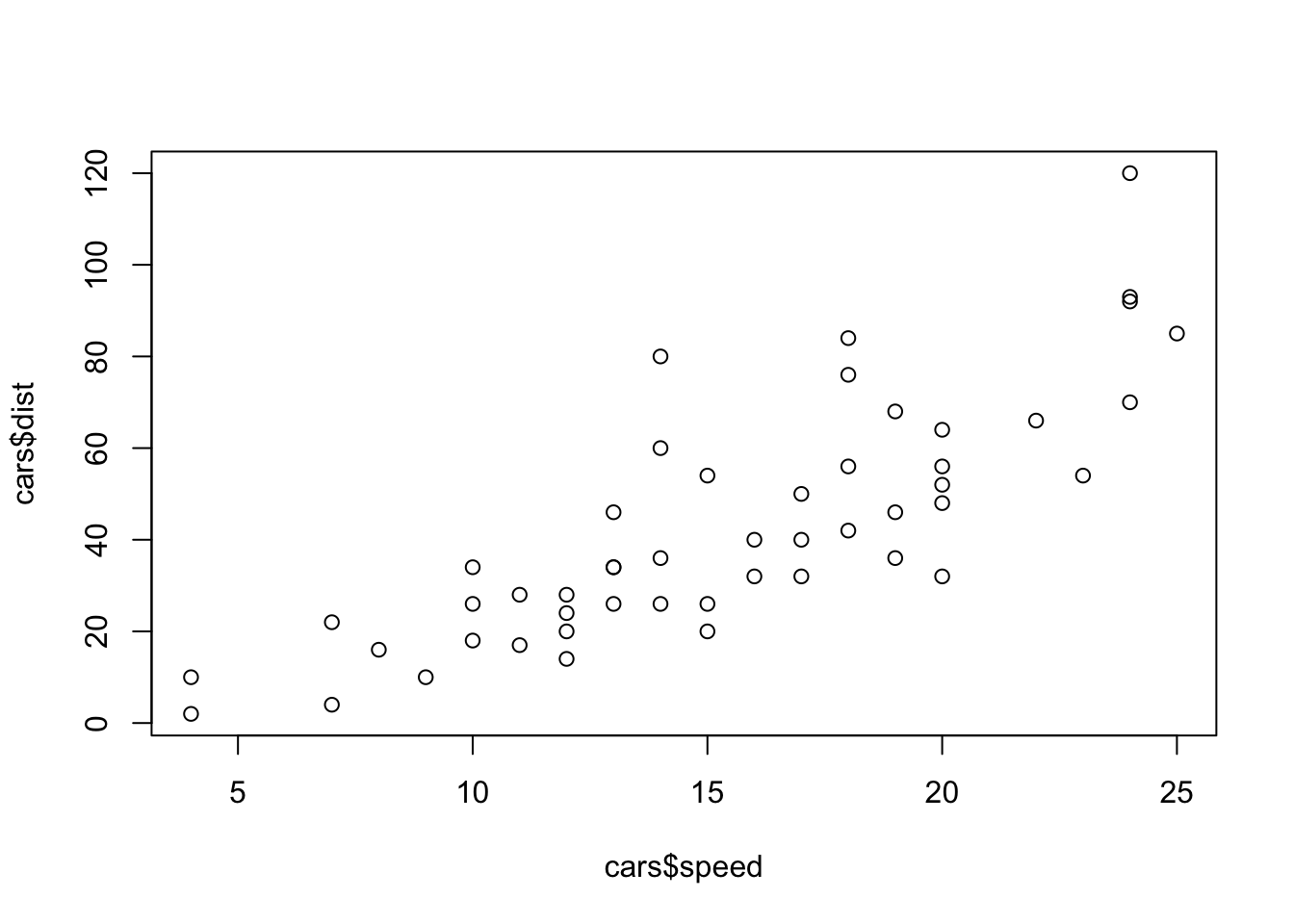
Embedding graphics created from R is also very easy.
plot(cars$speed, cars$dist)
Exercise
- Extend the template that creating Rmarkdown file with one more R command and one more graphic on cars dataset
Embedding graphics created from external programs is also straight forward. There are many ways to do it (for example using the  as noted above), but I prefer the following approach.
library(knitr) # include_graphics is a command in knitr package. We need to explictly initialise it once per session using the library command.
include_graphics("./img/anaconda.png") # Change the file path suitably.

Figure 1: An external image
Reading real data into R
In this course, we are going to follow the tidyverse style of programming and its associated packages. To read a comma separated file (*.csv) we are going to use read_csv command from tidyverse package.
Download the latest building violations data from building violations data from the Chicago Open Data Portal. For convenience, a local copy downloaded in 2019 is stored here.
library(tidyverse)


chicago_df <- read_csv(here('data', 'raw_data', 'Building_violations.csv'))
summary(chicago_df)
#        ID          VIOLATION LAST MODIFIED DATE VIOLATION DATE
#  Min.   : 219970   Length:1682199               Length:1682199
#  1st Qu.:2846372   Class :character             Class :character
#  Median :4173309   Mode  :character             Mode  :character
#  Mean   :4041069
#  3rd Qu.:5328152
#  Max.   :6404250
#
#  VIOLATION CODE     VIOLATION STATUS   VIOLATION STATUS DATE
#  Length:1682199     Length:1682199     Length:1682199
#  Class :character   Class :character   Class :character
#  Mode  :character   Mode  :character   Mode  :character
#
#
#
#
#  VIOLATION DESCRIPTION VIOLATION LOCATION VIOLATION INSPECTOR COMMENTS
#  Length:1682199        Length:1682199     Length:1682199
#  Class :character      Class :character   Class :character
#  Mode  :character      Mode  :character   Mode  :character
#
#
#
#
#  VIOLATION ORDINANCE INSPECTOR ID       INSPECTION NUMBER  INSPECTION STATUS
#  Length:1682199      Length:1682199     Min.   :  265575   Length:1682199
#  Class :character    Class :character   1st Qu.: 2306938   Class :character
#  Mode  :character    Mode  :character   Median :10422051   Mode  :character
#                                         Mean   : 8062623
#                                         3rd Qu.:11692850
#                                         Max.   :13061126
#
#  INSPECTION WAIVED  INSPECTION CATEGORY DEPARTMENT BUREAU    ADDRESS
#  Length:1682199     Length:1682199      Length:1682199     Length:1682199
#  Class :character   Class :character    Class :character   Class :character
#  Mode  :character   Mode  :character    Mode  :character   Mode  :character
#
#
#
#
#  STREET NUMBER   STREET DIRECTION   STREET NAME        STREET TYPE
#  Min.   :    1   Length:1682199     Length:1682199     Length:1682199
#  1st Qu.: 1648   Class :character   Class :character   Class :character
#  Median : 3746   Mode  :character   Mode  :character   Mode  :character
#  Mean   : 4151
#  3rd Qu.: 6229
#  Max.   :13770
#
#  PROPERTY GROUP        SSA             LATITUDE       LONGITUDE
#  Min.   :  1000   Min.   : 1.0      Min.   :41.64   Min.   :-87.91
#  1st Qu.: 20560   1st Qu.:22.0      1st Qu.:41.77   1st Qu.:-87.71
#  Median :154437   Median :34.0      Median :41.85   Median :-87.67
#  Mean   :202155   Mean   :33.8      Mean   :41.85   Mean   :-87.67
#  3rd Qu.:367135   3rd Qu.:49.0      3rd Qu.:41.91   3rd Qu.:-87.63
#  Max.   :678027   Max.   :69.0      Max.   :42.02   Max.   :-87.52
#                   NA's   :1359814   NA's   :1513    NA's   :1513
#    LOCATION
#  Length:1682199
#  Class :character
#  Mode  :character
#
#
#
#

nrow(chicago_df)
# [1] 1682199

str(chicago_df)
# spc_tbl_ [1,682,199 × 26] (S3: spec_tbl_df/tbl_df/tbl/data.frame)
#  $ ID                          : num [1:1682199] 3282077 1721274 1551698 1551137 1551226 ...
#  $ VIOLATION LAST MODIFIED DATE: chr [1:1682199] "10/14/2009" "10/24/2006" "05/14/2008" "08/11/2006" ...
#  $ VIOLATION DATE              : chr [1:1682199] "10/07/2009" "10/10/2006" "08/07/2006" "08/07/2006" ...
#  $ VIOLATION CODE              : chr [1:1682199] "CN198019" "CN198019" "PL159027" "CN069034" ...
#  $ VIOLATION STATUS            : chr [1:1682199] "OPEN" "OPEN" "COMPLIED" "OPEN" ...
#  $ VIOLATION STATUS DATE       : chr [1:1682199] NA NA "05/13/2008" NA ...
#  $ VIOLATION DESCRIPTION       : chr [1:1682199] "FILE BLDG REGISTRATION" "FILE BLDG REGISTRATION" "RESET LOOSE FIXTURE" "REPAIR AREAWAY WALL" ...
#  $ VIOLATION LOCATION          : chr [1:1682199] NA NA "BL00947 CRT" NA ...
#  $ VIOLATION INSPECTOR COMMENTS: chr [1:1682199] NA "BUILDING NOT REGISTERED 2005-06" "RESET LOOSE FIXTURE TOILET APARTMENT 3N" "REAR AREAWAY WALLS COLLAPSING INWARD" ...
#  $ VIOLATION ORDINANCE         : chr [1:1682199] "File building registration statement with Building Dept. (13-10-030, 13-10-040)" "File building registration statement with Building Dept. (13-10-030, 13-10-040)" "Reset loose plumbing fixture.  (18-29-102.3)" "Failed to maintain areaway walls in sound condition and good repair.  (13-196-530, 13-196-530(b), 13-196-641)" ...
#  $ INSPECTOR ID                : chr [1:1682199] "BL00873" "BL00878" "BL00947" "BL00875" ...
#  $ INSPECTION NUMBER           : num [1:1682199] 2811514 1135854 1528412 1426083 1426083 ...
#  $ INSPECTION STATUS           : chr [1:1682199] "CLOSED" "FAILED" "FAILED" "FAILED" ...
#  $ INSPECTION WAIVED           : chr [1:1682199] "N" "N" "N" "N" ...
#  $ INSPECTION CATEGORY         : chr [1:1682199] "COMPLAINT" "PERIODIC" "PERIODIC" "PERIODIC" ...
#  $ DEPARTMENT BUREAU           : chr [1:1682199] "DEMOLITION" "CONSERVATION" "CONSERVATION" "CONSERVATION" ...
#  $ ADDRESS                     : chr [1:1682199] "3918 S WELLS ST" "747 E 65TH ST" "6431 S COTTAGE GROVE AVE" "6431 S COTTAGE GROVE AVE" ...
#  $ STREET NUMBER               : num [1:1682199] 3918 747 6431 6431 6431 ...
#  $ STREET DIRECTION            : chr [1:1682199] "S" "E" "S" "S" ...
#  $ STREET NAME                 : chr [1:1682199] "WELLS" "65TH" "COTTAGE GROVE" "COTTAGE GROVE" ...
#  $ STREET TYPE                 : chr [1:1682199] "ST" "ST" "AVE" "AVE" ...
#  $ PROPERTY GROUP              : num [1:1682199] 304205 19591 19612 19612 19612 ...
#  $ SSA                         : num [1:1682199] NA NA NA NA NA NA NA NA NA NA ...
#  $ LATITUDE                    : num [1:1682199] NA NA NA NA NA NA NA NA NA NA ...
#  $ LONGITUDE                   : num [1:1682199] NA NA NA NA NA NA NA NA NA NA ...
#  $ LOCATION                    : chr [1:1682199] NA NA NA NA ...
#  - attr(*, "spec")=
#   .. cols(
#   ..   ID = col_double(),
#   ..   `VIOLATION LAST MODIFIED DATE` = col_character(),
#   ..   `VIOLATION DATE` = col_character(),
#   ..   `VIOLATION CODE` = col_character(),
#   ..   `VIOLATION STATUS` = col_character(),
#   ..   `VIOLATION STATUS DATE` = col_character(),
#   ..   `VIOLATION DESCRIPTION` = col_character(),
#   ..   `VIOLATION LOCATION` = col_character(),
#   ..   `VIOLATION INSPECTOR COMMENTS` = col_character(),
#   ..   `VIOLATION ORDINANCE` = col_character(),
#   ..   `INSPECTOR ID` = col_character(),
#   ..   `INSPECTION NUMBER` = col_double(),
#   ..   `INSPECTION STATUS` = col_character(),
#   ..   `INSPECTION WAIVED` = col_character(),
#   ..   `INSPECTION CATEGORY` = col_character(),
#   ..   `DEPARTMENT BUREAU` = col_character(),
#   ..   ADDRESS = col_character(),
#   ..   `STREET NUMBER` = col_double(),
#   ..   `STREET DIRECTION` = col_character(),
#   ..   `STREET NAME` = col_character(),
#   ..   `STREET TYPE` = col_character(),
#   ..   `PROPERTY GROUP` = col_double(),
#   ..   SSA = col_double(),
#   ..   LATITUDE = col_double(),
#   ..   LONGITUDE = col_double(),
#   ..   LOCATION = col_character()
#   .. )
#  - attr(*, "problems")=<externalptr>
Noticing that VIOLATION_DATE is stored as a character instead of a date, we fix it using mdy function from lubridate. This function is appropriate compared to another one such as ymd because the dates appear to be in month, day, year format.
library(lubridate)
chicago_df$`VIOLATION DATE` <- mdy(chicago_df$`VIOLATION DATE`)
Looking at the data gives you a lot information about how the data is read and stored. You will find that quirks of data types and storage produce many unexpected results. Pay close attention to this step to avoid countless hours of debugging. For example, why is Latitude and Longitude represented as T/F rather than a number?
Exercise
-
It is useful to develop specific naming conventions for variables and datasets, so that your code will be legible to you later on.
- Notice that column names have spaces in them. Rename the columns replacing the space with an underscore, using
renamecommand from tidyverse package - Notice that VIOLATION DATE column is read in as a character but should really be a date. We used the base R way to convert it into a date. However, if we were to follow a tidyverse way of doing it, how would you do it using
mutateandmdy? - Notice that parsing the file resulted in a lot of errors that read_csv gracefully skipped over. Examine the data file to understand what these errors are. Can you read the file correctly, by explicitly specifying the
col_typesin read_csv command. See help for read_csv. How would you access the help file?
- Notice that column names have spaces in them. Rename the columns replacing the space with an underscore, using
-
Set up a separate project and directory structure to read in the gasoline purchase data. Notice that there are 2 files (csv and xlsx). Read in both files and compare them. Which one is easier to read in? Why? Hint: You might have to use a different package (e.g.
openxlsx2) thantidyverseto read in the xlsx file.
Basic Data Manipulation
To find out the different violations issued by different bureaus and their status, we can create a contingency table using the table function.
chicago_cont_table_df <- table(chicago_df$`DEPARTMENT BUREAU`, chicago_df$`VIOLATION STATUS`)
chicago_cont_table_df
#
#                              COMPLIED NO ENTRY   OPEN
#   BOILER                        24690        0   6605
#   CONSERVATION                 425176     5591 683412
#   CONSTRUCTION EQUIPMENT          526        0     40
#   DEMOLITION                    11919        0 113397
#   ELECTRICAL                    17386        0  19927
#   ELEVATOR                      57378        0  28860
#   IRON                           5590        0   8779
#   NEW CONSTRUCTION               8070        0  22008
#   PLUMBING                      10626        0  17719
#   REFRIGERATION                 12552        0  17170
#   SIGNS                           976        0  13615
#   SPECIAL INSPECTION PROGRAM    11895        0   9229
#   SPECIAL TASK FORCE            40246        0  75743
#   VENTILATION                   18439        0  13847
#   WATER                           275        0    513
$ is special function that allows us access to the columns in a dataset. We use `` to access columns whose names have spaces or other special characters. Note that R is sensitive to capitalisation.
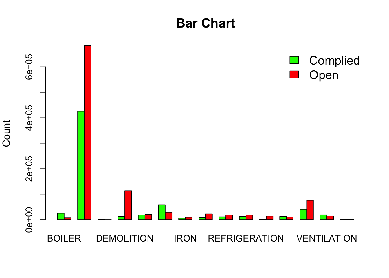
Notice that “No Entry” category is not relevant for most categories, so we ignore those records and create a barplot of this table.
chicago_df2 <- chicago_df[chicago_df$`VIOLATION STATUS` != "NO ENTRY",] #!=  is logical operator meaning not equal to.
chicago_cont_table_df2 <- table(chicago_df2$`VIOLATION STATUS`, chicago_df2$`DEPARTMENT BUREAU`) # Notice the flip from before. This is done to make the barplot work.

colrs <- c("Green","Red")

barplot(as.matrix(chicago_cont_table_df2 ), main="Bar Chart", ylab = "Count", cex.lab = 1.1, cex.main = 1.4, beside=TRUE, col= colrs)
legend("topright", c("Complied", "Open"), cex=1.3, bty="n", fill=colrs)
Exercise
The above is a terrible graphic and is used for demonstration purposes only. What is wrong with this graphic?
We can also subset the dataset by restricting it to 2008-2009 and write it out a separate dataset
chicago_df %>%
  filter(year(`VIOLATION DATE`) >= 2008 & year(`VIOLATION DATE`) < 2009) %>% #This will only work if you successfully used mdy function to convert VIOLATION DATE into a date format, instead of a character
  write_csv("../../../tutorials_datasets/buildingviolations/violations_2008.csv")
Notice few things that are important.
-
%>%is called a pipe operator. A combination function \(f(g(x))\) where \(f\) and \(g\) are functions and \(x\) is the argument can be written asx %>% f() %>% g(). You will do well to get comfortable with this pipe operator as it makes the code cleaner. It is part ofmagittrpackage, which is loaded when you calllibrary(tidyverse)in the earlier section of the code. See this tutorial for details. -
In newer versions of R (> 4.2.0), there is an alternative pipe operator
|>that is part of thebasepackage. In this course, I will switch between%>%and|>. You can use either one, but you might want to be mindful of the crucial differences between%>%and|>. -
&is a logical operator.&and&&indicate logical AND and|and||indicate logical OR. The shorter form performs element wise comparisons in much the same way as arithmetic operators. The longer form evaluates left to right examining only the first element of each vector. Evaluation proceeds only until the result is determined. The longer form is appropriate for programming control-flow and typically preferred in if clauses. -
I could have simply used year(.) == 2008 to achieve the same result. But in what situations will this code fail to do what you want it to do? Hint: 2008 could be stored and interpreted in R in lot of different ways (double, character, Date).
-
filteris function from tidyverse that subsets the data by filter rows. A corresponding function that subsets columns is calledselect. -
write_csvis a function that writes a dataset into a csv file.
Exercise
-
The
write_csvfunction in the above code chunk uses bad programming practise. Rewrite that piece of code in more correct way using project workflow ideas andhere. -
In the gasoline purchases data set, write out a subset of the data that only contains purchases in the summer months. Use the project workflow ideas.
Now consider that you want to programmatically create subsets of this data by year for each year. You can repeat the above code numerous times, each time modifying the filter function and the file path in the write_csv function. Such procedure is tedious. Instead, we can write a function that takes year as a argument, and repeatedly call the function with the right argument.
write_chicago_df_fun <- function(yr){  #yr is an argument. Avoid using names that are already other functions, such as year.

  file_name_str <- paste(here('data', 'processed_data'), "/violations_", yr, ".csv", sep = "")
     # This will create a string "$PROJ_HOME/data/processed_data/violations_2008.csv" when yr == 2008 and store it in the variable "file_name_str" and so on. (with appropriate substitutions for PROJ_HOME that is unique to your computer)

   chicago_df %>%
  filter(year(`VIOLATION DATE`) == yr) %>%  # Note the ==
  write_csv(file_name_str)

  return() #return null, because we are already writing the dataset into a disk file.
}


for (yr2 in 2006:2020){  # I am using yr2 as a variable to avoid confusion between arguments.
  write_chicago_df_fun(yr2)
}
# Alternately, if you don't think that you will use the write_chicago_df_fun again, you can just write a loop

for (yr2 in 2006:2020){
 file_name_str <- paste(here('data', 'processed_data'), "/violations_", yr, ".csv", sep = "") #

  chicago_df %>%
  filter(year(`VIOLATION DATE`) == yr2) %>%  # Note the yr2
  write_csv(file_name_str)

  rm(file_name_str) #It is a good practise to clean up after yourself.
}
You should see all the files correctly labelled as below

Exercise
-
Notice that I included 2020 in the loop and R faithfully produced an empty file called
violations_2020.csv. While this is innocuous at the moment, user errors might create unexpected results. Add some error checking to the function and trap these situations. Do not simply change the for loop condition. -
Adapt the function and the for loop to write out files in two year increments e.g.
violations_2006_2007.csvandviolations_2008_2009.csv -
Can you find a more R way to replace the for loop? Hint: use
map -
Repeat similar steps for the gasoline purchases project.
Additional Resources
Nikhil Kaza
Professor
My research interests include urbanization patterns, local energy policy and equity