Basic Raster Operations in R

Introduction
While much of urban data systems moved to vector object based data structures, raster datasets are ubiquitous and ever present. Raster datasets are simply an array of pixels/cells organized into rows and columns (or a grid) where each cell contains a value representing information, such as temperature, soil type, land use, water level. Rasters are aerial photographs, imagery from satellites, google street view images.
Few things to note:
- Raster datasets are always rectangular (rows x col) similar to matrices. Irregular boundaries and holes are created by using NAs.
- Rasters have to contain values of the same type (int, float, boolean) throughout the raster, just like matrices and unlike data.frames
- The size of the raster depends on the resolution and the extent of the raster. As such many rasters are large and often cannot be held in memory completely.
- In general, rasters we would interested in have a coordinate system (projected or unprojected). Because of it regular nature of the data structure, all we need to store is the Origin coordinates and the cell resolution (square or rectangular).
Rasters in R
The workhorse packages for working with rasters in R is raster and terra packages by Robert Hijmans. In particular see Spatial Data Science with R. terra is better and faster in many instances, but is newer and does not have all the functionality and support associated with raster. I will switch back and forth between the two packages as necessary. Most functions are available in both packages, but it is useful to learn the differences
Eventually, if you get into the weeds in Remote Sensing, you should use RStoolbox package that has support for parallel processing. If you are working in rasters that are not geographically located (such as digital pictures) magick wrapper around ImageMagick may be a good option.
Download data
You can download the datasets used in this tutorial here
Reading in Rasters
Let’s start with toy examples and examine the use of functions in the raster and terra packages.
library(raster)
library(rasterVis)
library(sf)
library(tidyverse)
library(tigris)
library(leaflet)
library(skimr)
library(terra)
# Let's create a raster of size 5x5. #creates an empty raster object
raster_object <- raster(ncol=5, nrow=5, xmx=-100, xmn=-500, ymn=100, ymx=500, crs='+proj=longlat +datum=WGS84')
#In terra, you can create an object with 'rast'. Notice the difference between xmx and xmax argument names.
raster_object_terra <- rast(ncol=5, nrow=5, xmax=-100, xmin=-500, ymin=100, ymax=500, crs='+proj=longlat +datum=WGS84')
#view its properties
raster_object
# class : RasterLayer
# dimensions : 5, 5, 25 (nrow, ncol, ncell)
# resolution : 80, 80 (x, y)
# extent : -500, -100, 100, 500 (xmin, xmax, ymin, ymax)
# crs : +proj=longlat +datum=WGS84 +no_defs
raster_object_terra
# class : SpatRaster
# size : 5, 5, 1 (nrow, ncol, nlyr)
# resolution : 80, 80 (x, y)
# extent : -500, -100, 100, 500 (xmin, xmax, ymin, ymax)
# coord. ref. : +proj=longlat +datum=WGS84 +no_defs
#access the resolution of the object
res(raster_object)
# [1] 80 80
#we can also set the resolution of the object
res(raster_object) <- 100
res(raster_object)
# [1] 100 100
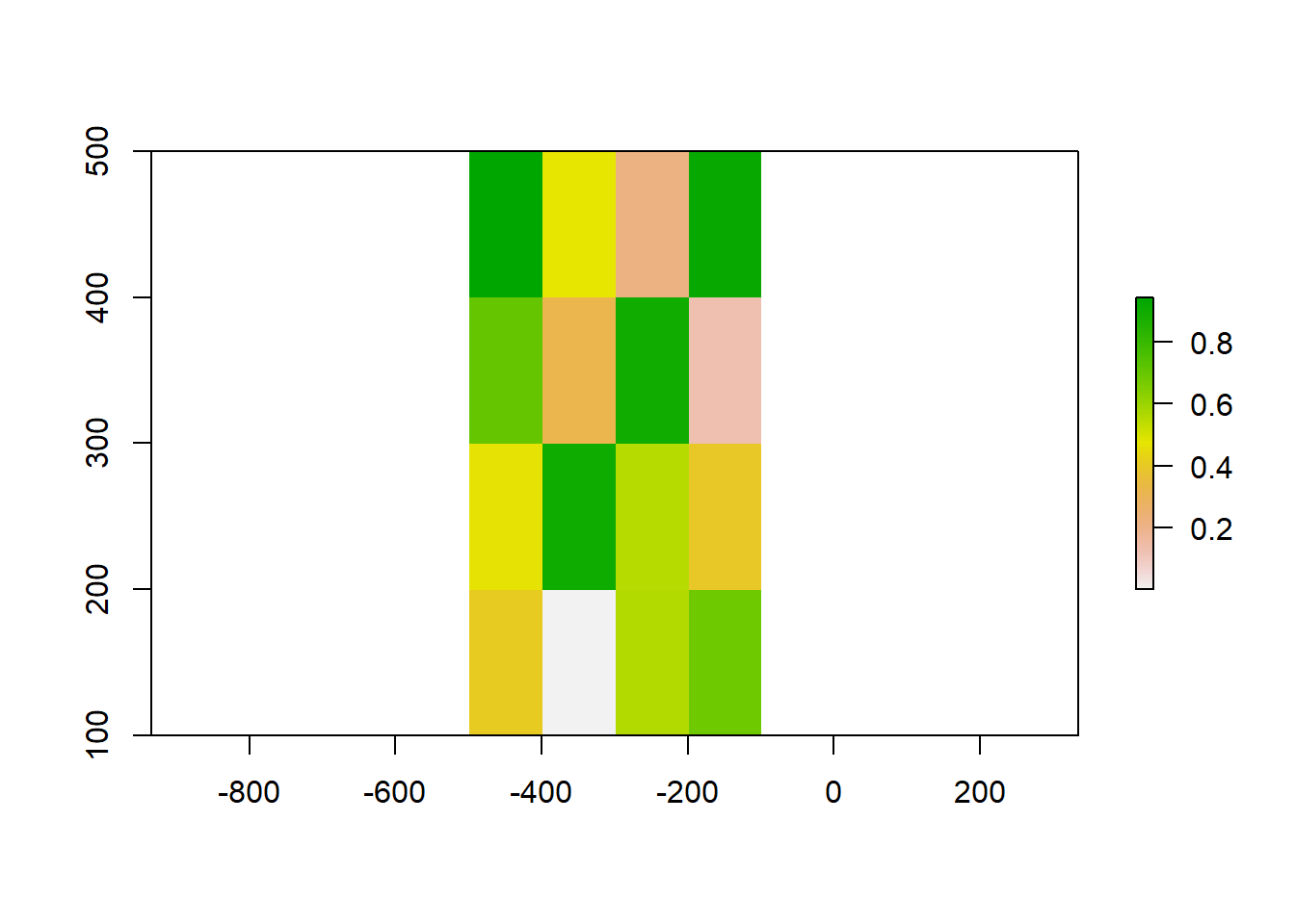
# We can assign values to the object by supplying the right number of values.
values(raster_object) <- runif(ncell(raster_object))
plot(raster_object)
# Basic airthmetic is treated as
raster_object2 <- raster_object * 2
Exercise
- Notice the difference in the format between objects created by
rastandraster. Read up on those differences.
Of course, the real advantage is to reading in rasters that we can work with in the urban policy arena. Rasters come in many formats.
Say for example, we want to read in tree cover data in the ERDAS Imagine (*.img) format.
library(here)


(durham_treecover_raster <- here("tutorials_datasets", "basicraster", "durham_treecover.img") %>% raster)
# class      : RasterLayer
# dimensions : 1483, 888, 1316904  (nrow, ncol, ncell)
# resolution : 30, 30  (x, y)
# extent     : 1510245, 1536885, 1558875, 1603365  (xmin, xmax, ymin, ymax)
# crs        : +proj=aea +lat_0=23 +lon_0=-96 +lat_1=29.5 +lat_2=45.5 +x_0=0 +y_0=0 +ellps=GRS80 +units=m +no_defs
# source     : durham_treecover.img
# names      : Layer_1
# values     : 0, 100  (min, max)


# Download the boundary of the county for visualisation purposes.

durhamcty_sf <- counties(state = 37, refresh=TRUE, cb=TRUE, progress_bar = FALSE) %>%
                  st_as_sf() %>%
                  filter(GEOID == "37063") %>%
                  st_transform(crs = crs(durham_treecover_raster))
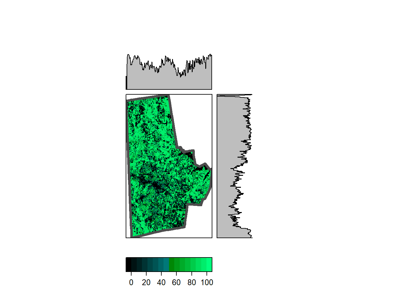
Note that the durham_treecover_raster only is a reference to a file and not loaded fully into memory. Also note the resolution, origin and dimensions. The tree cover is also an integer raster with values ranging from 0 to 100. Integers take up fewer bytes than floats and doubles, in general. The raster can be visualised as a static plot or in leaflet.
rasterVis::levelplot(durham_treecover_raster,
                     ylab=NULL, xlab=NULL,
                     scales=list(y=list(draw=FALSE), x=list(draw=FALSE)),
                     col.regions = rgb(0,0:100/100,0:50/100),
                     margin = list(FUN = 'median')
                     ) +
  latticeExtra::layer(sp.lines(as(durhamcty_sf, "Spatial"), col="gray30", lwd=4))
library(widgetframe)

leaflet() %>%
  addRasterImage(durham_treecover_raster, layerId = "values", colors = colorNumeric("Greens", domain = 0:100)) %>%
  leafem::addMouseCoordinates() %>%
 # leafem::addImageQuery(durham_treecover_raster, type="click", layerId = "values") %>%  # looks like broken in leafem.
  frameWidget()
RasterLayer not SpatRaster.
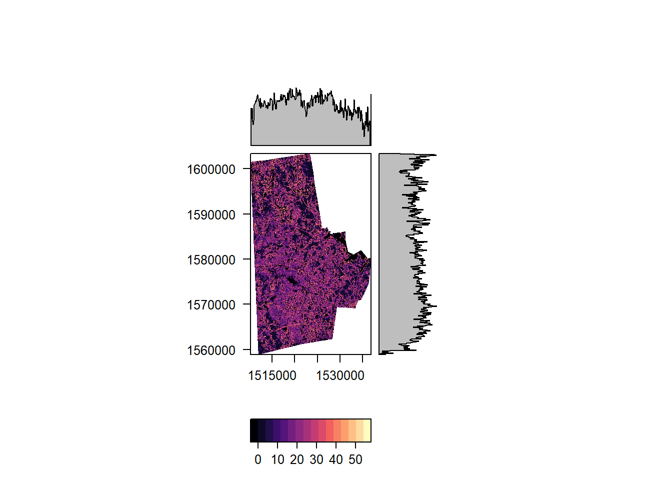
In addition to visualisation we can process the entire raster or use a focal window. The first bit provides the median of all the values of the raster (removing NAs automatically) and the second creates a raster, whose value is the the median in 3x3 window around the focal cell. Note that we have treat NAs explicitly in the focal operations.
cellStats(durham_treecover_raster, "sd", asSample = FALSE)
# [1] 39.14223

durham_treecover_focal <- focal(durham_treecover_raster, w = matrix(1, nrow = 3, ncol = 3), fun = function(x,...){sd(x,na.rm=TRUE)})

# leaflet() %>%
#   addRasterImage(durham_treecover_focal, layerId = "values", colors = colorNumeric("Greens", domain = 0:70)) %>%
#   leafem::addMouseCoordinates() %>%
#  # leafem::addImageQuery(durham_treecover_focal, type="mousemove", layerId = "values") %>% # Looks like this is broken in leafem. see https://github.com/r-spatial/leafem/issues/7
#   frameWidget()

rasterVis::levelplot(durham_treecover_focal)
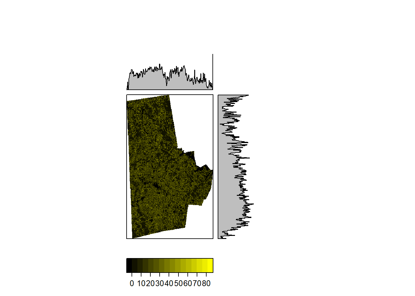
More complicated functions are certainly possible. The following takes the average of the deviation all the cells in the 3x3 neighborhood w.r.t. the value of the focal cell.
unevenness_raster <- focal(durham_treecover_raster, w=matrix(1, nrow=3, ncol=3), fun=function(x, ...) sum(abs(x[-5]-x[5]))/8, pad=TRUE, padValue=NA)

rasterVis::levelplot(unevenness_raster,
                     ylab=NULL, xlab=NULL,
                     scales=list(y=list(draw=FALSE), x=list(draw=FALSE)),
                     col.regions = rgb(0:100/100,0:100/100,0),
                     margin = list(FUN = 'median')
)
** Exercise **
- Use a different window (neighborhood) and calculate the focal values.
- Use a different function to summarize the values. How are cells on the edge treated, with lot of the neighbors being NAs?
Vectors & Rasters
In addition to raster based windows, we can use vector based neighborhoods and calculate the statistics (or any other metric). The only difference is that in a focal operation, the windows move over the raster cell by cell, where as zonal operations are exclusive, i.e. if a cell belongs to a zone, it is does not belong to another zone. For example, the following code calculates the Median and Interquartile ranges in each tract of Durham and stores them per tract.
This is where terra shines. I am going to convert the Rasterlayer to SpatRaster and proceed. However, terra requires the vector layer to be in its proprietary format. Fortunately, vect easily converts an sf object to a vect object.
durham_tracts_sf <- tracts(state='37', county='063', progress_bar = FALSE, year='2010') %>%
  st_as_sf() %>%
  st_transform(crs = crs(durham_treecover_raster))


durham_treecover_terra <- rast(durham_treecover_raster)

tree_bg <- terra::extract(durham_treecover_terra, vect(durham_tracts_sf))

tree_bg_summary <-tree_bg %>%
                    group_by(ID) %>%
                    dplyr::summarise(treecover_iqr = IQR(Layer_1, na.rm=T),
                                      treecover_median = median(Layer_1, na.rm=T))


durham_tracts_sf <- cbind(durham_tracts_sf, tree_bg_summary) # Can do this because extract uses the record ID and we have not scrambled the sf object. Use with caution. See further down for a better method

durham_tracts_sf %>%
  st_set_geometry(NULL) %>%
  dplyr::select(treecover_median, treecover_iqr) %>%
  skim
| Name | Piped data |
| Number of rows | 60 |
| Number of columns | 2 |
| _______________________ | |
| Column type frequency: | |
| numeric | 2 |
| ________________________ | |
| Group variables | None |
Table 1: Data summary
Variable type: numeric
| skim_variable | n_missing | complete_rate | mean | sd | p0 | p25 | p50 | p75 | p100 | hist |
|---|---|---|---|---|---|---|---|---|---|---|
| treecover_median | 0 | 1 | 46.20 | 24.92 | 0 | 31 | 45.5 | 65.5 | 92 | ▃▅▇▃▃ |
| treecover_iqr | 0 | 1 | 61.33 | 20.29 | 0 | 48 | 62.0 | 79.0 | 94 | ▁▂▇▇▇ |
Exercise
- Notice the output differences when you use
raster::extractandterra::extract.- Modify the code so that you can merge with the sf object.
- Run microbenchmarks on these two functions and see which is faster and more efficient. Also think about the collection of functions to get to the output and run the microbenchmarks. Bottlenecks can be in different places.
Categorical Rasters
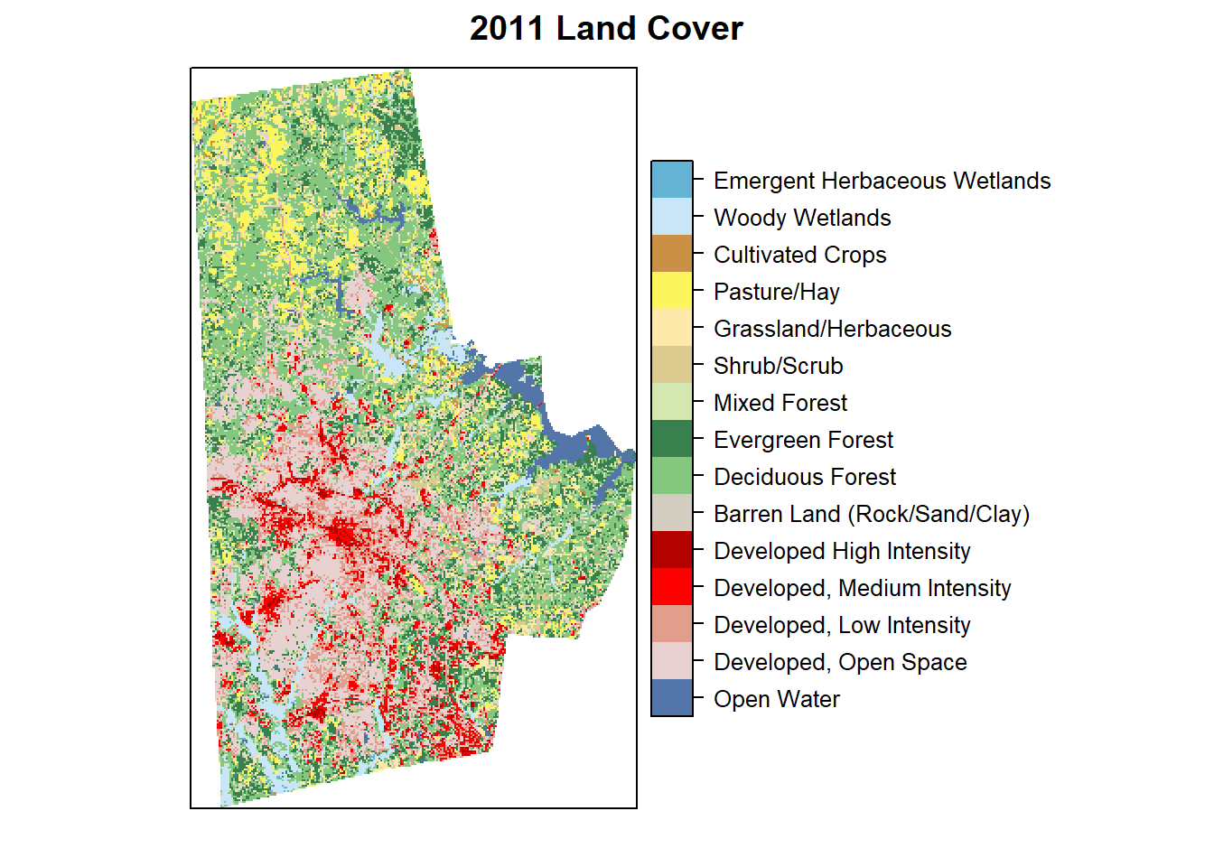
Some times raster can be categorical (nominal or ordinal values), however, they are stored as numbers for convenience just as factors in regular R. For example a land cover raster might have a value 21 representing Developed Open Space and 95 representing Emergent Wetlands. While it is certainly possible to do arithmetic on them (additions and subtractions etc.), those operations do not make substantive sense. Explicit care should be taken to analyse these categorical rasters.
In particular, use ratify function to create a Raster Attribute Table and use it for analyses and visualisation as below.
durham_lc_raster <- here("tutorials_datasets", "basicraster", "c11_37063.img") %>%
                  raster() %>%
                  ratify()


nlcd_class <- here("tutorials_datasets", "basicraster", "legend_csv.csv") %>%
              read_csv()


rat <- levels(durham_lc_raster)[[1]] %>% merge(nlcd_class, by.x="ID", by.y="Value")

levels(durham_lc_raster) <- rat

levelplot(durham_lc_raster, att="Classification", ylab=NULL, xlab=NULL, scales=list(y=list(draw=FALSE), x=list(draw=FALSE)),  col.regions=levels(durham_lc_raster)[[1]]$colortable, main="2011 Land Cover")
We can also extract all cells with in each polygon and produce counts using the table function. Confirm to make sure that the projections and vectors and rasters are the same.
proj4string(durham_lc_raster)
# [1] "+proj=aea +lat_0=23 +lon_0=-96 +lat_1=29.5 +lat_2=45.5 +x_0=0 +y_0=0 +ellps=GRS80 +units=m +no_defs"
crs(durham_tracts_sf)
# [1] "PROJCRS[\"unknown\",\n    BASEGEOGCRS[\"unknown\",\n        DATUM[\"Unknown based on GRS 1980 ellipsoid\",\n            ELLIPSOID[\"GRS 1980\",6378137,298.257222101,\n                LENGTHUNIT[\"metre\",1],\n                ID[\"EPSG\",7019]]],\n        PRIMEM[\"Greenwich\",0,\n            ANGLEUNIT[\"degree\",0.0174532925199433],\n            ID[\"EPSG\",8901]]],\n    CONVERSION[\"unknown\",\n        METHOD[\"Albers Equal Area\",\n            ID[\"EPSG\",9822]],\n        PARAMETER[\"Latitude of false origin\",23,\n            ANGLEUNIT[\"degree\",0.0174532925199433],\n            ID[\"EPSG\",8821]],\n        PARAMETER[\"Longitude of false origin\",-96,\n            ANGLEUNIT[\"degree\",0.0174532925199433],\n            ID[\"EPSG\",8822]],\n        PARAMETER[\"Latitude of 1st standard parallel\",29.5,\n            ANGLEUNIT[\"degree\",0.0174532925199433],\n            ID[\"EPSG\",8823]],\n        PARAMETER[\"Latitude of 2nd standard parallel\",45.5,\n            ANGLEUNIT[\"degree\",0.0174532925199433],\n            ID[\"EPSG\",8824]],\n        PARAMETER[\"Easting at false origin\",0,\n            LENGTHUNIT[\"metre\",1],\n            ID[\"EPSG\",8826]],\n        PARAMETER[\"Northing at false origin\",0,\n            LENGTHUNIT[\"metre\",1],\n            ID[\"EPSG\",8827]]],\n    CS[Cartesian,2],\n        AXIS[\"(E)\",east,\n            ORDER[1],\n            LENGTHUNIT[\"metre\",1,\n                ID[\"EPSG\",9001]]],\n        AXIS[\"(N)\",north,\n            ORDER[2],\n            LENGTHUNIT[\"metre\",1,\n                ID[\"EPSG\",9001]]]]"

durham_lc_terra <- rast(durham_lc_raster)
extract from terra conflicts with the same function from raster, so it is useful to explicitly specify the package the function comes from.
Furthermore, extract relies on on the record number or row number. It is useful to create a new table with the row number and an ID column like GEOID10 which can then be used to merge back.
tract_geoid <- tibble(ID = 1:nrow(durham_tracts_sf), GEOID10 = durham_tracts_sf$GEOID10)


lc_tracts <- terra::extract(durham_lc_terra, vect(durham_tracts_sf)) %>%
              mutate(Layer_1 = paste0("lc", Layer_1)) %>% # This is an easy way to convert to characters and therefore to factors. Layer_1 and ID are columns in the tibble that results from from terra::extract
              group_by(ID, Layer_1)  %>%
              summarize(count = n())

lc_tracts_tbl <- lc_tracts %>%
                 ungroup() %>% # Groups are no longer necessary
                  pivot_wider(names_from = Layer_1, values_from = count) %>%
                  left_join(tract_geoid)

lc_tracts_tbl
# # A tibble: 60 × 17
#       ID  lc11  lc21  lc22  lc23  lc24  lc41  lc42  lc43  lc52  lc71  lc81  lc90
#    <dbl> <int> <int> <int> <int> <int> <int> <int> <int> <int> <int> <int> <int>
#  1     1    35  3994  2233   790   176  1373  1139   224    91   175    72     7
#  2     2     9  4099   633   276    22   371   308    79     1    18    NA   854
#  3     3    NA   429   618   249   253    NA    NA    NA    NA    NA    NA    NA
#  4     4  3907 12486  2371   723   209 85032 25850  8729  5115 11342 39446  7882
#  5     5    NA   690   950   859   157    51    17    NA    NA    NA    NA    NA
#  6     6  9776  4085   755   412    76 25189 15132  4238  3421  5364  4986  1674
#  7     7    NA  2517   566   458   156    41    NA    35    NA     7    NA    NA
#  8     8   914  5732  1114   212     5 12414  2242   919   565  1498  2801  1371
#  9     9   153  6603   731   108    NA 11765  3395  1670   381   952  1489    75
# 10    10   130  5958  1996  1387   224  3112  2519   410   105   369   308  3490
# # ℹ 50 more rows
# # ℹ 4 more variables: lc31 <int>, lc82 <int>, lc95 <int>, GEOID10 <chr>
Tips & Tricks
Exploit RasterOptions
There are two parameters that have a lot of influence on the performance of the package: chunksize and maxmemory.
- chunksize: integer. Maximum number of cells to read/write in a single chunk while processing (chunk by chunk) disk based Raster* objects
- maxmemory: integer. Maximum number of cells to read into memory.
You can override the default values using rasterOptions(maxmemory = 1e+09). Other options that are useful to set within rasterOptions are overwrite and datatype
Parallelise your operations
While rasters are large, you can take advantage of the fact that not all operations have to be sequential and can be done in parallel.
- Use
clusterRto parallelize some operations such ascalc,overlayandpredict. - Use
foreachanddoParallelpackages whenever possible.
Manage your temp files
When multiple operations are run on rasters, because they need to written to disk often, they create multiple copies of the same raster. This quickly takes up space and stops the script from moving forward. Use removeTmpFiles(h=) to periodically empty tempfiles. It is always a good idea to set temporary directory using tempdir() at the beginning of the script and then unlink() to delete the directory at the end of the script.
Conclusions
Rasters are incredibly useful in urban domains but are often left to remote sensing experts. In the next few tutorials we will see how they can be used to characterise urban form and identify suitable sites. They should sit along side with vector data manipulation in the analysts’ toolbox.
Nikhil Kaza
Professor
My research interests include urbanization patterns, local energy policy and equity