Spatial Data in R

Nikhil Kaza

2026-09-15

Today’s plan

  • Thinking about space
  • sf for storing and processing spatial objects
  • tmap for visualising spatial objects
  • Advanced R with sf
  • Further work

Thinking about space

Conceptual rethink

Spatial is just a data type (mostly…)

library(tidyverse)
library(here)

sm_tbl <-
    here("data", "201806-citibike-tripdata.csv") %>%
    read_csv()
  •   Nearly 2 million trips
  •   776 bike-share station locations
  •   11,888 unique bikes
BikeID tripid station_name_D station_name_O lon_D lon_O lat_D lat_O dat_time_D dat_time_O
21481 1 Broadway & W 49 St W 52 St & 11 Ave -73.98453 -73.99393 40.76068 40.76727 2018-06-01 02:06:50 2018-06-01 01:57:20
19123 2 W 41 St & 8 Ave W 52 St & 11 Ave -73.99003 -73.99393 40.75641 40.76727 2018-06-01 02:10:43 2018-06-01 02:02:42
26983 3 Broadway & W 58 St W 52 St & 11 Ave -73.98169 -73.99393 40.76695 40.76727 2018-06-01 02:15:55 2018-06-01 02:04:23
26742 4 W 31 St & 7 Ave W 52 St & 11 Ave -73.99160 -73.99393 40.74916 40.76727 2018-06-01 03:11:59 2018-06-01 03:00:55
26386 5 W 20 St & 11 Ave W 52 St & 11 Ave -74.00776 -73.99393 40.74674 40.76727 2018-06-01 06:18:32 2018-06-01 06:04:54
27073 6 W 24 St & 7 Ave W 52 St & 11 Ave -73.99530 -73.99393 40.74488 40.76727 2018-06-01 06:24:26 2018-06-01 06:11:52

Spatial is just a data type (mostly…)

library(tidyverse)
library(here)

sm_tbl <-
    here("data", "201806-citibike-tripdata.csv") %>%
    read_csv() %>%
    rename(
        station_name_O = `start station name`,
        station_name_D = `end station name`,
        lon_O = `start station longitude`,
        lat_O = `start station latitude`,
        lon_D = `end station longitude`,
        lat_D = `end station latitude`,
        dat_time_O = starttime,
        dat_time_D = stoptime,
        BikeID = bikeid
    )
BikeID tripid station_name_D station_name_O lon_D lon_O lat_D lat_O dat_time_D dat_time_O
21481 1 Broadway & W 49 St W 52 St & 11 Ave -73.98453 -73.99393 40.76068 40.76727 2018-06-01 02:06:50 2018-06-01 01:57:20
19123 2 W 41 St & 8 Ave W 52 St & 11 Ave -73.99003 -73.99393 40.75641 40.76727 2018-06-01 02:10:43 2018-06-01 02:02:42
26983 3 Broadway & W 58 St W 52 St & 11 Ave -73.98169 -73.99393 40.76695 40.76727 2018-06-01 02:15:55 2018-06-01 02:04:23
26742 4 W 31 St & 7 Ave W 52 St & 11 Ave -73.99160 -73.99393 40.74916 40.76727 2018-06-01 03:11:59 2018-06-01 03:00:55
26386 5 W 20 St & 11 Ave W 52 St & 11 Ave -74.00776 -73.99393 40.74674 40.76727 2018-06-01 06:18:32 2018-06-01 06:04:54
27073 6 W 24 St & 7 Ave W 52 St & 11 Ave -73.99530 -73.99393 40.74488 40.76727 2018-06-01 06:24:26 2018-06-01 06:11:52

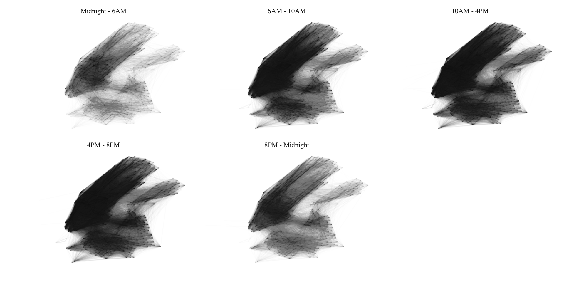
Visualising spatial data

Code
library(ggplot2)
library(ggthemes)

numtrips <- sm_tbl %>%
    filter(station_name_O != station_name_D) %>%
  mutate(hr = hour(dat_time_O),
         time_of_day = hr %>% cut(breaks=c(0,6,10,16,20,24), include.lowest = TRUE, labels=c("Midnight - 6AM", "6AM - 10AM", "10AM - 4PM", "4PM - 8PM", "8PM - Midnight"))
         ) %>%
  group_by(station_name_O, station_name_D, time_of_day) %>%
  summarise(lon_O = first(lon_O),
            lat_O = first(lat_O),
            lon_D = first(lon_D),
            lat_D = first(lat_D),
            totaltrips = n()
            )


numtrips %>%
 ggplot()+
  geom_segment(aes(x=lon_O, y=lat_O,xend=lon_D, yend=lat_D, alpha=totaltrips))+
  #Here is the magic bit that sets line transparency - essential to make the plot readable
  scale_alpha_continuous(trans = "log10", range = c(0.005, 0.04), guide='none')+
  facet_wrap(time_of_day~.)+
  #Set black background, ditch axes
  scale_x_continuous("", breaks=NULL)+
  scale_y_continuous("", breaks=NULL) +
    theme_tufte()
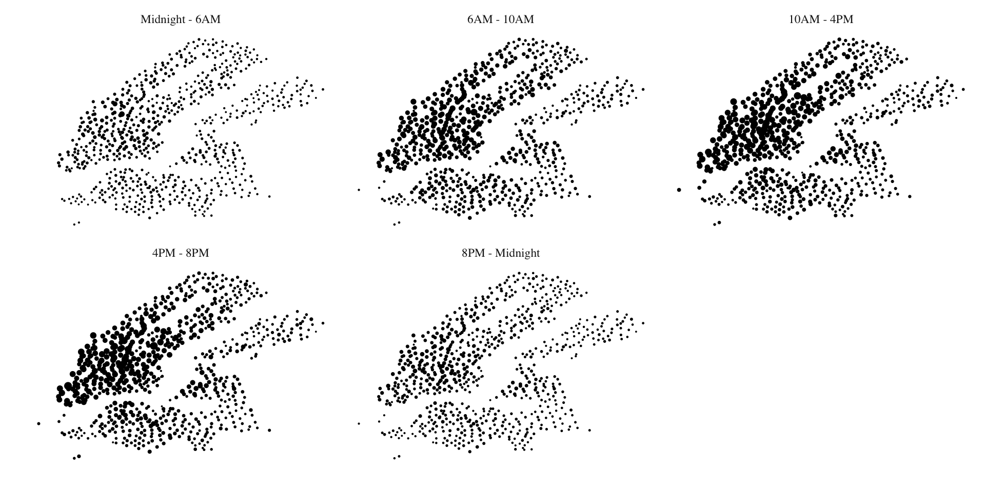
Visualising spatial data differently (O)

Code
numtrips <- sm_tbl %>%
    filter(station_name_O != station_name_D) %>%
  mutate(hr = hour(dat_time_O),
         time_of_day = hr %>% cut(breaks=c(0,6,10,16,20,24), include.lowest = TRUE, labels=c("Midnight - 6AM", "6AM - 10AM", "10AM - 4PM", "4PM - 8PM", "8PM - Midnight"))
         ) %>%
  group_by(station_name_O, time_of_day) %>%
  summarise(lon_O = first(lon_O),
            lat_O = first(lat_O),
            totaltrips = n()
            )


numtrips %>%
 ggplot()+
  geom_point(aes(x=lon_O, y=lat_O, size=totaltrips))+
  scale_size_continuous(range = c(0.01, 2), guide='none')+
  facet_wrap(time_of_day~.)+
  #Set black background, ditch axes
  scale_x_continuous("", breaks=NULL)+
  scale_y_continuous("", breaks=NULL) +
    theme_tufte()+
    labs(main = "Popularity of origin stations, June 2018")
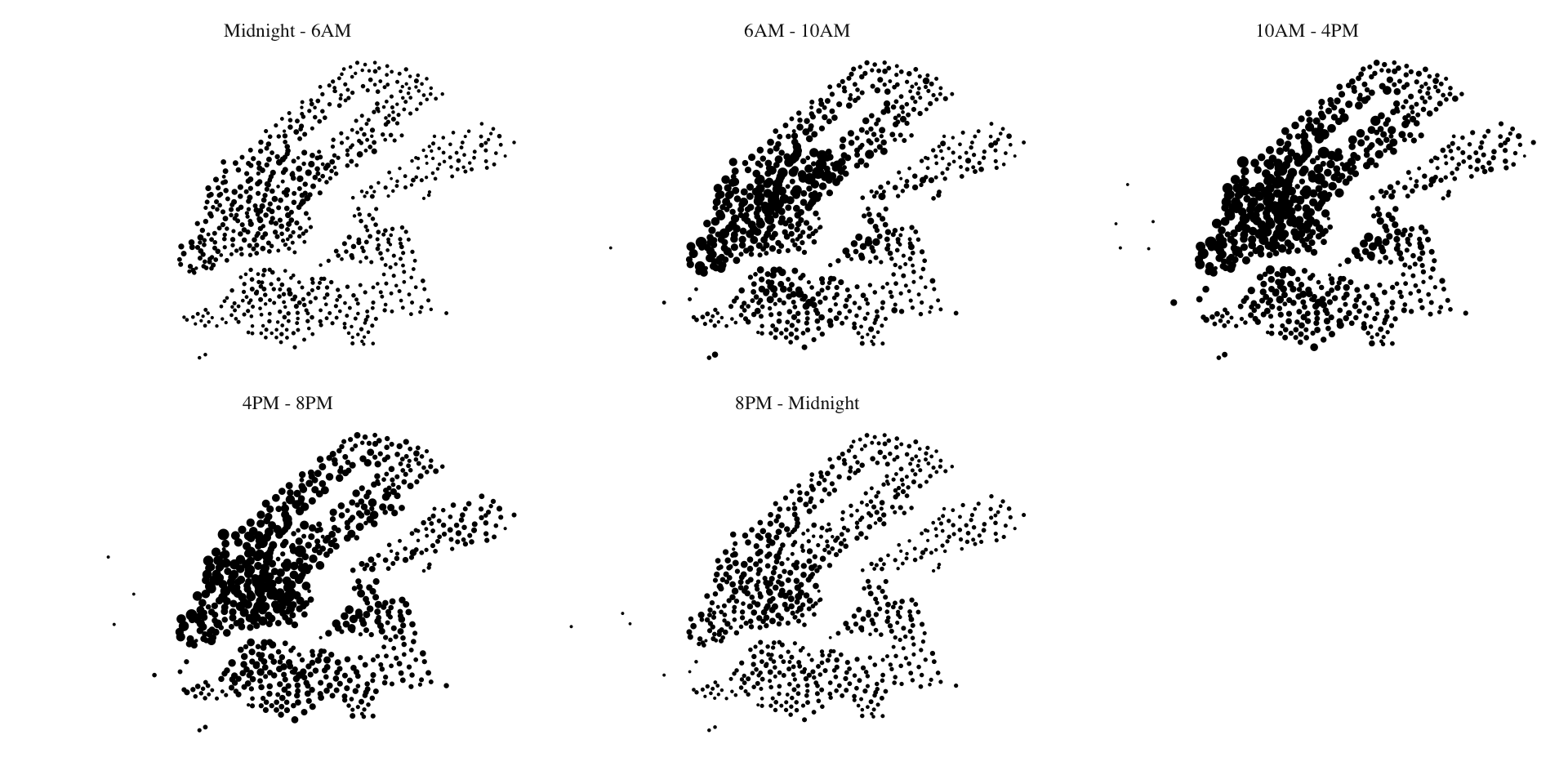
Visualising spatial data differently (D)

Code
numtrips <- sm_tbl %>%
    filter(station_name_O != station_name_D) %>%
  mutate(hr = hour(dat_time_O),
         time_of_day = hr %>% cut(breaks=c(0,6,10,16,20,24), include.lowest = TRUE, labels=c("Midnight - 6AM", "6AM - 10AM", "10AM - 4PM", "4PM - 8PM", "8PM - Midnight"))
         ) %>%
  group_by(station_name_D, time_of_day) %>%
  summarise(lon_D = first(lon_D),
            lat_D = first(lat_D),
            totaltrips = n()
            )


numtrips %>%
 ggplot()+
  geom_point(aes(x=lon_D, y=lat_D, size=totaltrips))+
  scale_size_continuous(range = c(0.01, 2), guide='none')+
  facet_wrap(time_of_day~.)+
  #Set black background, ditch axes
  scale_x_continuous("", breaks=NULL)+
  scale_y_continuous("", breaks=NULL) +
    theme_tufte()+
    labs(main = "Popularity of destination stations, June 2018")
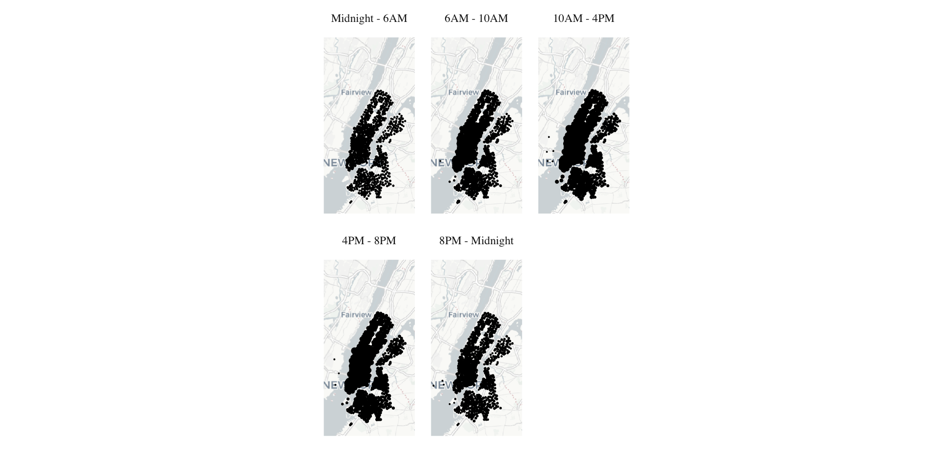
But basemaps provide context

Code
library(maptiles)
library(terra)
library(tidyterra)

bbox <- c(left = -74.06, bottom = 40.64, right = -73.89, top = 40.89)
bbox_sf <- sf::st_bbox(c(xmin = unname(bbox["left"]), ymin = unname(bbox["bottom"]),
                         xmax = unname(bbox["right"]), ymax = unname(bbox["top"])), crs = 4326) %>%
    sf::st_as_sfc()
g1 <- get_tiles(bbox_sf, provider = carto_positron, zoom = 10, crop = TRUE, apikey = carto_key)


ggplot() +
    geom_spatraster_rgb(data = g1) +
    geom_point(aes(x=lon_D, y=lat_D, size=totaltrips), data = numtrips)+
  scale_size_continuous(range = c(0.01, 2), guide='none')+
  facet_wrap(time_of_day~.)+
  #Set black background, ditch axes
  scale_x_continuous("", breaks=NULL)+
  scale_y_continuous("", breaks=NULL) +
    theme_tufte()
Easier with tmap (but need to get serious)

Code
library(tmap)
tmap_mode("view")

sm_tbl %>%
    distinct(lon_D, lat_D) %>%
    drop_na %>%
    sf::st_as_sf(coords = c("lon_D", "lat_D"), crs = 4326) %>%
    tm_shape()+
    tm_dots(fill = "red", size = .5)+
    tm_basemap(carto_tile_url, sub = "abcd")

Introducing sf

Spatial with sf

Spatial with sf

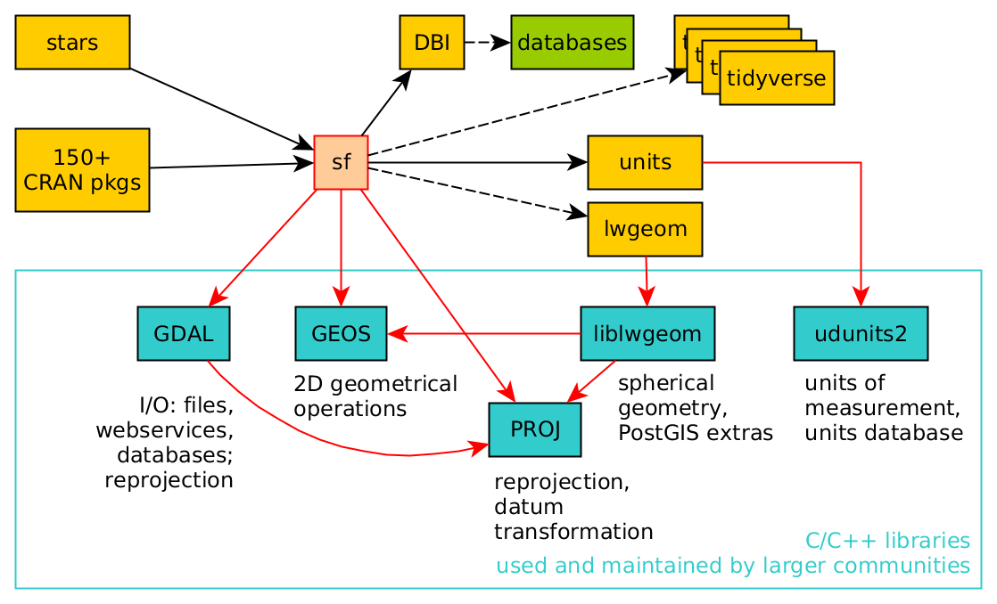
  • represents simple features as records with a geometry list-column
  • represents natively in R all 17 simple feature types for all dimensions (XY, XYZ, XYM, XYZM)
  • interfaces to GEOS (projected) and s2geometry (unprojected)
  • interfaces to GDAL, supporting all driver options
  • reads from and writes to spatial databases such as PostGIS using DBI

sf ecosystem

sf: Objects with simple features
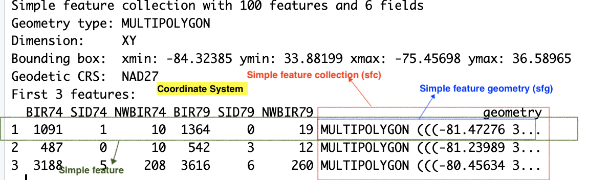
library(sf)
nc <- st_read(system.file("shape/nc.shp", package="sf"))
print(nc[9:15], n = 3)

Geometry

Polygons are complex (A digression)

Geometry is not that different from time
Promote a set of columns to a geometry column

scard_sf <- sm_tbl %>%
    drop_na(lon_D, lat_D) %>%
    sf::st_as_sf(coords = c("lon_D", "lat_D"), crs = 4326)
BikeID tripid station_name_D station_name_O lon_O lat_O dat_time_D dat_time_O geometry
21481 1 Broadway & W 49 St W 52 St & 11 Ave -73.99393 40.76727 2018-06-01 02:06:50 2018-06-01 01:57:20 POINT (-73.98453 40.76068)
19123 2 W 41 St & 8 Ave W 52 St & 11 Ave -73.99393 40.76727 2018-06-01 02:10:43 2018-06-01 02:02:42 POINT (-73.99003 40.75641)
26983 3 Broadway & W 58 St W 52 St & 11 Ave -73.99393 40.76727 2018-06-01 02:15:55 2018-06-01 02:04:23 POINT (-73.98169 40.76695)
26742 4 W 31 St & 7 Ave W 52 St & 11 Ave -73.99393 40.76727 2018-06-01 03:11:59 2018-06-01 03:00:55 POINT (-73.9916 40.74916)
26386 5 W 20 St & 11 Ave W 52 St & 11 Ave -73.99393 40.76727 2018-06-01 06:18:32 2018-06-01 06:04:54 POINT (-74.00776 40.74674)
27073 6 W 24 St & 7 Ave W 52 St & 11 Ave -73.99393 40.76727 2018-06-01 06:24:26 2018-06-01 06:11:52 POINT (-73.9953 40.74488)

Be careful with sticky geometry

scard_sf %>%
    filter(BikeID == 14656) %>%
    select(station_name_O)
station_name_O geometry
Willoughby St & Fleet St POINT (-73.98433 40.68021)
Adelphi St & Myrtle Ave POINT (-73.9813 40.69197)
Douglass St & 4 Ave POINT (-73.97632 40.68383)
Douglass St & 3 Ave POINT (-73.97945 40.66106)

Multiple sets of columns are good candidates for geometry

scard_sf <- sm_tbl %>%
                    sf::st_as_sf(coords = c("lon_D", "lat_D"), crs = 4326) 

scard_sf$orig_geom <- sm_tbl %>%
                    sf::st_as_sf(coords = c("lon_O", "lat_O"), crs = 4326) %>%
                    st_geometry()                   
BikeID tripid geometry orig_geom
21481 1 POINT (-73.98453 40.76068) POINT (-73.99393 40.76727)
19123 2 POINT (-73.99003 40.75641) POINT (-73.99393 40.76727)
26983 3 POINT (-73.98169 40.76695) POINT (-73.99393 40.76727)
26742 4 POINT (-73.9916 40.74916) POINT (-73.99393 40.76727)
26386 5 POINT (-74.00776 40.74674) POINT (-73.99393 40.76727)
27073 6 POINT (-73.9953 40.74488) POINT (-73.99393 40.76727)

Create new geometries

scard_sf %>%
    mutate(buffer_geom = st_buffer(orig_geom, .05))
BikeID orig_geom buffer_geom geometry
21481 POINT (-73.99393 40.76727) POLYGON ((-73.99393 40.7672... POINT (-73.98453 40.76068)
19123 POINT (-73.99393 40.76727) POLYGON ((-73.99393 40.7672... POINT (-73.99003 40.75641)
26983 POINT (-73.99393 40.76727) POLYGON ((-73.99393 40.7672... POINT (-73.98169 40.76695)
26742 POINT (-73.99393 40.76727) POLYGON ((-73.99393 40.7672... POINT (-73.9916 40.74916)
26386 POINT (-73.99393 40.76727) POLYGON ((-73.99393 40.7672... POINT (-74.00776 40.74674)
27073 POINT (-73.99393 40.76727) POLYGON ((-73.99393 40.7672... POINT (-73.9953 40.74488)

A reminder that (only active) geometry is sticky

scard_sf %>%
    select(station_name_D, dat_time_D) 
station_name_D dat_time_D geometry
Broadway & W 49 St 2018-06-01 02:06:50 POINT (-73.98453 40.76068)
W 41 St & 8 Ave 2018-06-01 02:10:43 POINT (-73.99003 40.75641)
Broadway & W 58 St 2018-06-01 02:15:55 POINT (-73.98169 40.76695)
W 31 St & 7 Ave 2018-06-01 03:11:59 POINT (-73.9916 40.74916)

Use plyrs

scard_sf %>%
   filter(station_name_O != station_name_D) %>%
  mutate(hr = hour(dat_time_O),
         time_of_day = hr %>% cut(breaks=c(0,6,10,16,20,24), include.lowest = TRUE, labels=c("Midnight - 6AM", "6AM - 10AM", "10AM - 4PM", "4PM - 8PM", "8PM - Midnight"))
         )
BikeID tripid hr time_of_day geometry
21481 1 1 Midnight - 6AM POINT (-73.98453 40.76068)
19123 2 2 Midnight - 6AM POINT (-73.99003 40.75641)
26983 3 2 Midnight - 6AM POINT (-73.98169 40.76695)
26742 4 3 Midnight - 6AM POINT (-73.9916 40.74916)
26386 5 6 Midnight - 6AM POINT (-74.00776 40.74674)
27073 6 6 Midnight - 6AM POINT (-73.9953 40.74488)

… but worry about summarisation

scard_sf %>%
   filter(station_name_O != station_name_D) %>%
  mutate(hr = hour(dat_time_O),
         time_of_day = hr %>% cut(breaks=c(0,6,10,16,20,24), include.lowest = TRUE, labels=c("Midnight - 6AM", "6AM - 10AM", "10AM - 4PM", "4PM - 8PM", "8PM - Midnight"))
         ) %>%
    group_by(time_of_day) %>%
    summarise(totaltrips = n())
totaltrips time_of_day geometry
6 Midnight - 6AM MULTIPOINT ((-73.99003 40.7...
32 6AM - 10AM MULTIPOINT ((-74.00278 40.7...
12 10AM - 4PM MULTIPOINT ((-73.99667 40.7...

Drop it!

scard_sf %>%
    st_drop_geometry()
BikeID tripid station_name_D station_name_O lon_O lat_O dat_time_D dat_time_O orig_geom
21481 1 Broadway & W 49 St W 52 St & 11 Ave -73.99393 40.76727 2018-06-01 02:06:50 2018-06-01 01:57:20 POINT (-73.99393 40.76727)
19123 2 W 41 St & 8 Ave W 52 St & 11 Ave -73.99393 40.76727 2018-06-01 02:10:43 2018-06-01 02:02:42 POINT (-73.99393 40.76727)
26983 3 Broadway & W 58 St W 52 St & 11 Ave -73.99393 40.76727 2018-06-01 02:15:55 2018-06-01 02:04:23 POINT (-73.99393 40.76727)
26742 4 W 31 St & 7 Ave W 52 St & 11 Ave -73.99393 40.76727 2018-06-01 03:11:59 2018-06-01 03:00:55 POINT (-73.99393 40.76727)

Particularly useful in summarisation

scard_sf %>%
   filter(station_name_O != station_name_D) %>%
  mutate(hr = hour(dat_time_O),
         time_of_day = hr %>% cut(breaks=c(0,6,10,16,20,24), include.lowest = TRUE, labels=c("Midnight - 6AM", "6AM - 10AM", "10AM - 4PM", "4PM - 8PM", "8PM - Midnight"))
         ) %>%
    st_drop_geometry() %>%
    group_by(time_of_day) %>%
    summarise(totaltrips = n())
time_of_day totaltrips
Midnight - 6AM 91060
6AM - 10AM 425052
10AM - 4PM 649292
4PM - 8PM 601275
8PM - Midnight 143179

Visualisation with tmap

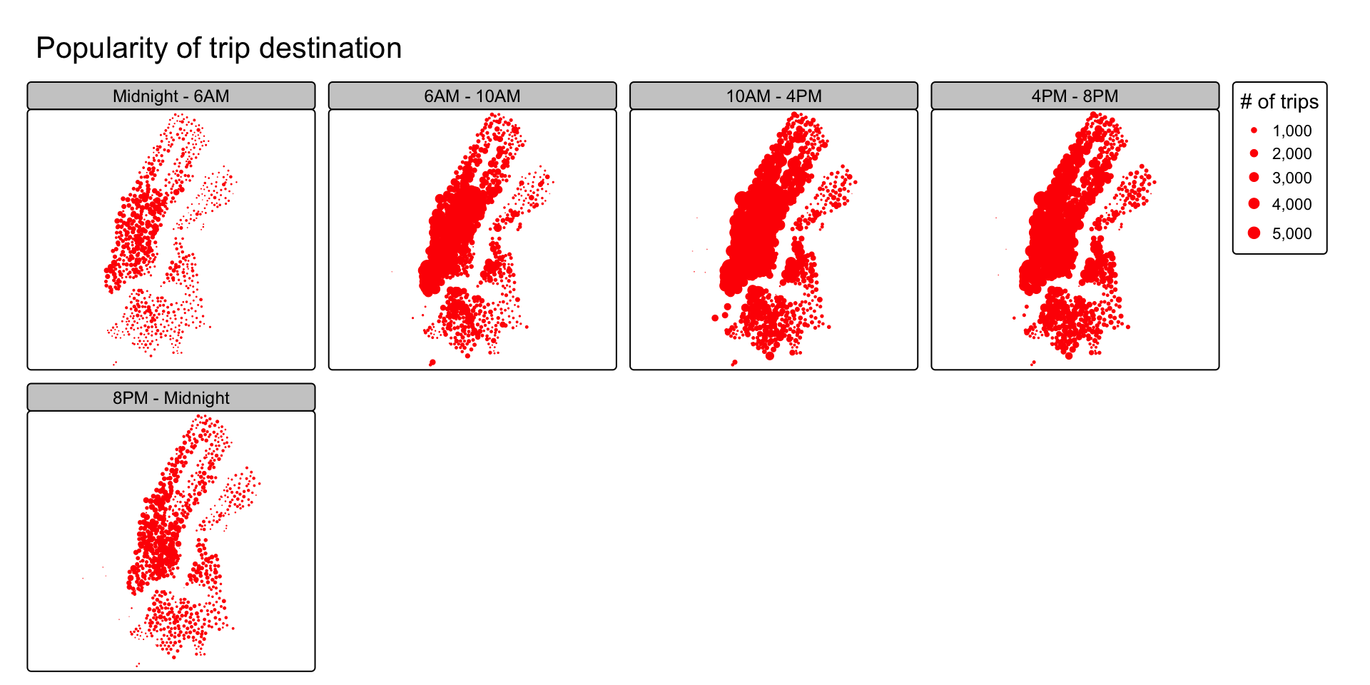
tmap again

Code
tmap_mode("plot")

numtrips <- sm_tbl %>%
    filter(station_name_O != station_name_D) %>%
  mutate(hr = hour(dat_time_O),
         time_of_day = hr %>% cut(breaks=c(0,6,10,16,20,24), include.lowest = TRUE, labels=c("Midnight - 6AM", "6AM - 10AM", "10AM - 4PM", "4PM - 8PM", "8PM - Midnight"))
         ) %>%
  group_by(station_name_D, time_of_day) %>%
  summarise(lon_D = first(lon_D),
            lat_D = first(lat_D),
            totaltrips = n()
            ) %>%
    st_as_sf(coords = c("lon_D", "lat_D"), crs=4326) 


numtrips %>%
    tm_shape()+
    tm_bubbles(size = "totaltrips", 
            col="red",
            border.col = "red",
            title.size = "# of trips",
            legend.size.is.portrait = TRUE
            )+
    tm_facets(by = "time_of_day") +
     tm_layout(
            legend.outside.size = 0.2,
            main.title= 'Popularity of trip destination', 
            main.title.position = c("center", 'top'))
tmap can create interactive maps

Code
tmap_mode('view')

numtrips %>%
    filter(time_of_day == "4PM - 8PM") %>%
    tm_shape(name = "Stations")+
    tm_bubbles(size = "totaltrips",
            col="red",
            border.col = "red",
            alpha = .5
            ) +
    tm_basemap(carto_tile_url, sub = "abcd")

Advanced R with sf

Perhaps the geometry needs to be different

scard_geom <- sm_tbl %>%
    select(lon_O, lat_O, lon_D, lat_D) %>% 
    split(seq(nrow(.))) %>%
    map(function(row){unlist(row) %>% matrix(ncol = 2, byrow=T) %>% st_linestring()}) %>%
    st_as_sfc(crs = 4326)

scard_sf_line <- st_sf(sm_tbl, scard_geom)
BikeID station_name_O station_name_D geometry
21481 W 52 St & 11 Ave Broadway & W 49 St LINESTRING (-73.99393 40.76...
19123 W 52 St & 11 Ave W 41 St & 8 Ave LINESTRING (-73.99393 40.76...
26983 W 52 St & 11 Ave Broadway & W 58 St LINESTRING (-73.99393 40.76...
26742 W 52 St & 11 Ave W 31 St & 7 Ave LINESTRING (-73.99393 40.76...
26386 W 52 St & 11 Ave W 20 St & 11 Ave LINESTRING (-73.99393 40.76...
27073 W 52 St & 11 Ave W 24 St & 7 Ave LINESTRING (-73.99393 40.76...

Let’s break it down (1)

sm_tbl %>%
    select(lon_O, lat_O, lon_D, lat_D) %>% 
    split(seq(nrow(.)))
$`1`
# A tibble: 1 × 4
  lon_O lat_O lon_D lat_D
  <dbl> <dbl> <dbl> <dbl>
1 -74.0  40.8 -74.0  40.8

$`2`
# A tibble: 1 × 4
  lon_O lat_O lon_D lat_D
  <dbl> <dbl> <dbl> <dbl>
1 -74.0  40.8 -74.0  40.8

$`3`
# A tibble: 1 × 4
  lon_O lat_O lon_D lat_D
  <dbl> <dbl> <dbl> <dbl>
1 -74.0  40.8 -74.0  40.8

$`4`
# A tibble: 1 × 4
  lon_O lat_O lon_D lat_D
  <dbl> <dbl> <dbl> <dbl>
1 -74.0  40.8 -74.0  40.7

$`5`
# A tibble: 1 × 4
  lon_O lat_O lon_D lat_D
  <dbl> <dbl> <dbl> <dbl>
1 -74.0  40.8 -74.0  40.7

$`6`
# A tibble: 1 × 4
  lon_O lat_O lon_D lat_D
  <dbl> <dbl> <dbl> <dbl>
1 -74.0  40.8 -74.0  40.7

Let’s break it down (2)

sm_tbl %>%
    select(lon_O, lat_O, lon_D, lat_D) %>% 
    split(seq(nrow(.))) %>%
    map(function(row){unlist(row) %>% matrix(ncol = 2, byrow=T) %>% st_linestring()}) 
$`1`
LINESTRING (-73.99393 40.76727, -73.98453 40.76068)

$`2`
LINESTRING (-73.99393 40.76727, -73.99003 40.75641)

$`3`
LINESTRING (-73.99393 40.76727, -73.98169 40.76695)

$`4`
LINESTRING (-73.99393 40.76727, -73.9916 40.74916)

$`5`
LINESTRING (-73.99393 40.76727, -74.00776 40.74674)

$`6`
LINESTRING (-73.99393 40.76727, -73.9953 40.74488)

Let’s break it down (2.1)

row <- tibble (lon_O = 121.364284201405, 
             lat_O = 31.1600086708404, 
             lon_D = 121.422563109174, 
             lat_D = 31.1885822807991)

unlist(row) %>% 
    matrix(ncol = 2, byrow=T)  
         [,1]     [,2]
[1,] 121.3643 31.16001
[2,] 121.4226 31.18858

Let’s break it down (2.2)

unlist(row) %>% 
    matrix(ncol = 2, byrow=T) %>%
    st_linestring()
LINESTRING (121.3643 31.16001, 121.4226 31.18858)

Let’s break it down (3)

sm_tbl %>%
    select(lon_O, lat_O, lon_D, lat_D) %>% 
    split(seq(nrow(.))) %>%
    map(function(row){unlist(row) %>% matrix(ncol = 2, byrow=T) %>% st_linestring()})  %>%
    st_as_sfc(crs = 4326)
Geometry set for 6 features 
Geometry type: LINESTRING
Dimension:     XY
Bounding box:  xmin: -74.00776 ymin: 40.74488 xmax: -73.98169 ymax: 40.76727
Geodetic CRS:  WGS 84
First 5 geometries:
LINESTRING (-73.99393 40.76727, -73.98453 40.76...
LINESTRING (-73.99393 40.76727, -73.99003 40.75...
LINESTRING (-73.99393 40.76727, -73.98169 40.76...
LINESTRING (-73.99393 40.76727, -73.9916 40.74916)
LINESTRING (-73.99393 40.76727, -74.00776 40.74...

Let’s break it down (4)

scard_geom <- sm_tbl %>%
    select(lon_O, lat_O, lon_D, lat_D) %>% 
    split(seq(nrow(.))) %>%
    map(function(row){unlist(row) %>% matrix(ncol = 2, byrow=T) %>% st_linestring()})  %>%
    st_as_sfc(crs = 4326)


scard_sf_line <- st_sf(sm_tbl, scard_geom)
BikeID station_name_O station_name_D geometry
21481 W 52 St & 11 Ave Broadway & W 49 St LINESTRING (-73.99393 40.76...
19123 W 52 St & 11 Ave W 41 St & 8 Ave LINESTRING (-73.99393 40.76...
26983 W 52 St & 11 Ave Broadway & W 58 St LINESTRING (-73.99393 40.76...
26742 W 52 St & 11 Ave W 31 St & 7 Ave LINESTRING (-73.99393 40.76...
26386 W 52 St & 11 Ave W 20 St & 11 Ave LINESTRING (-73.99393 40.76...
27073 W 52 St & 11 Ave W 24 St & 7 Ave LINESTRING (-73.99393 40.76...

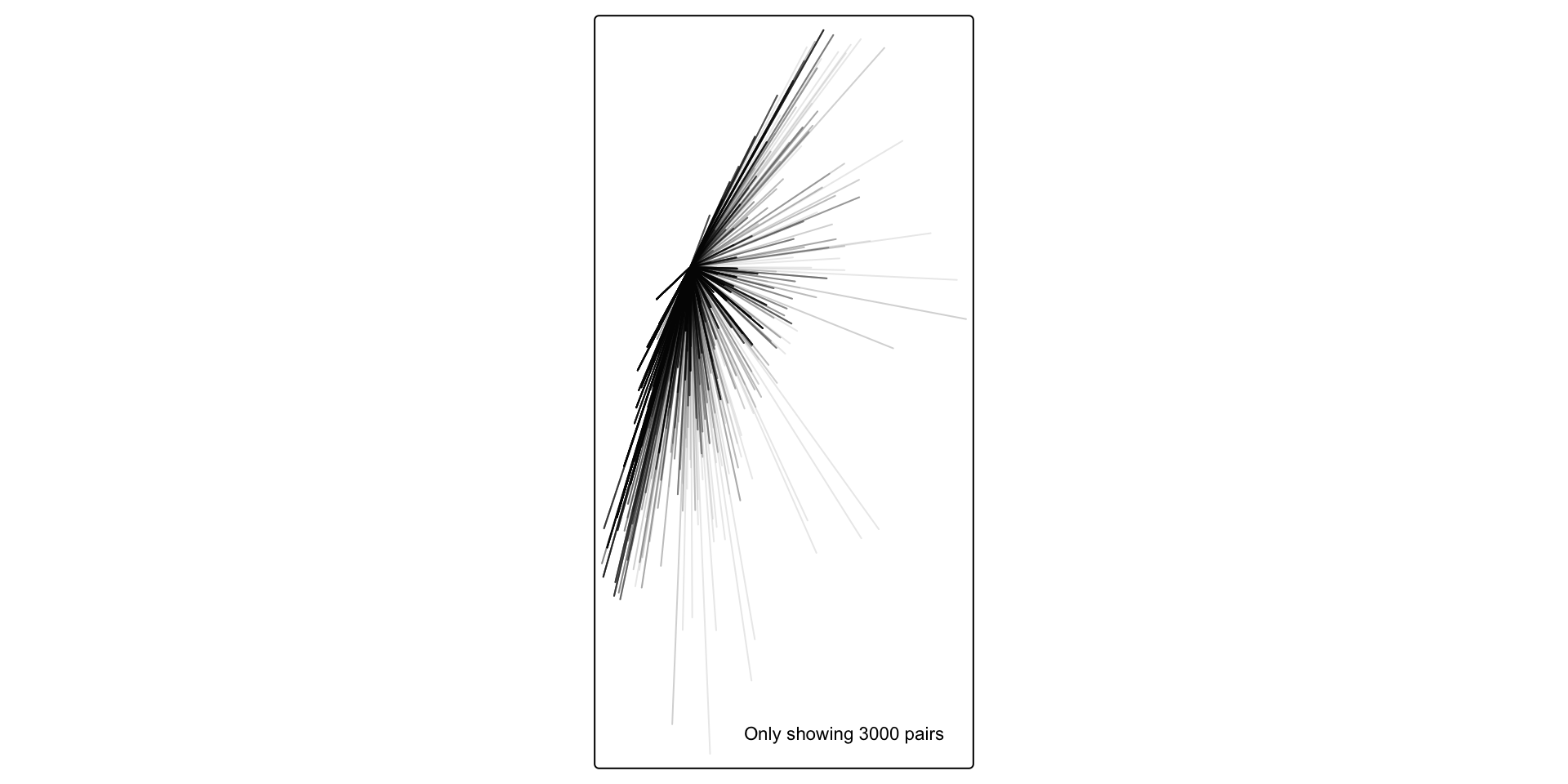
Visualise it

scard_sf_line %>%
   tm_shape(name = "OD pair") +
    tm_lines(alpha = .1) 

Just because you can doesn’t mean you should

  • Is that the right visualisation?
  • Was it informative? In what context?
  • What kind of information does it show and what does it obscure?
  • How else to convey information?

Reading in external spatial objects

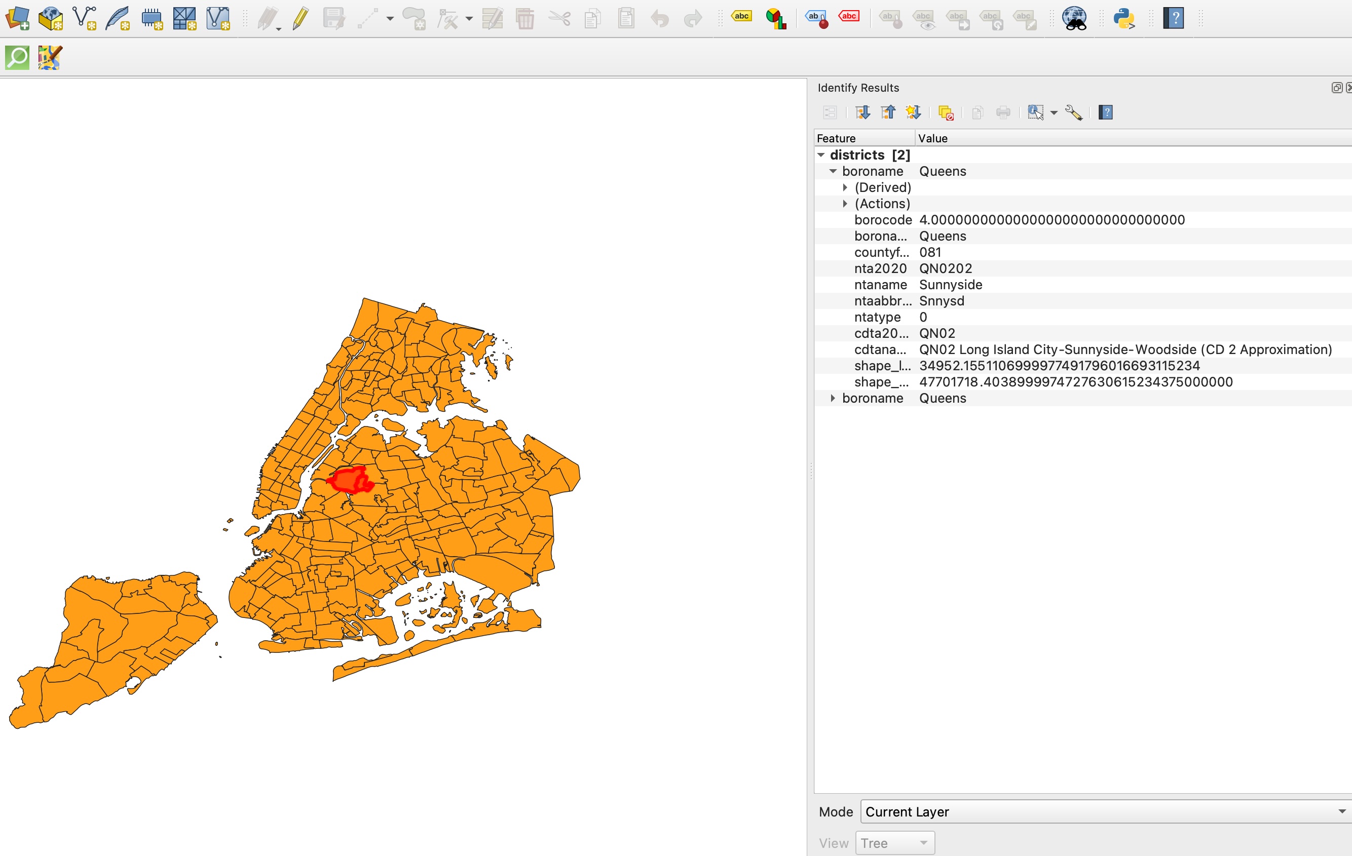
dist <- 
    here("static", "slides-src", "spatial_with_sf", "data", "districts.shp") %>%
    st_read()
Reading layer `districts' from data source 
  `/Users/kaza/Desktop/website_new/website/static/slides-src/spatial_with_sf/data/districts.shp' 
  using driver `ESRI Shapefile'
Simple feature collection with 262 features and 11 fields
Geometry type: MULTIPOLYGON
Dimension:     XY
Bounding box:  xmin: -74.25559 ymin: 40.49613 xmax: -73.70001 ymax: 40.91553
Geodetic CRS:  WGS 84
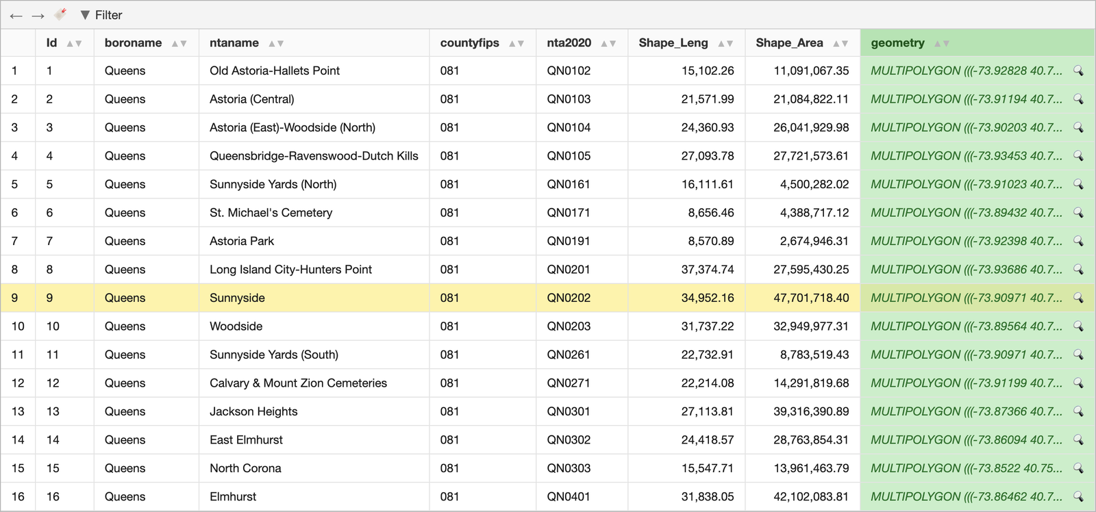
borocode boroname countyfips nta2020 ntaname ntaabbrev ntatype cdta2020 cdtaname shape_leng shape_area geometry
3 Brooklyn 047 BK0101 Greenpoint Grnpt 0 BK01 BK01 Williamsburg-Greenpoint (CD 1 Equivalent) 28919.56 35321808 MULTIPOLYGON (((-73.93213 4...
3 Brooklyn 047 BK0102 Williamsburg Wllmsbrg 0 BK01 BK01 Williamsburg-Greenpoint (CD 1 Equivalent) 28134.08 28852853 MULTIPOLYGON (((-73.95814 4...
3 Brooklyn 047 BK0103 South Williamsburg SWllmsbrg 0 BK01 BK01 Williamsburg-Greenpoint (CD 1 Equivalent) 18250.28 15208961 MULTIPOLYGON (((-73.95024 4...
3 Brooklyn 047 BK0104 East Williamsburg EWllmsbrg 0 BK01 BK01 Williamsburg-Greenpoint (CD 1 Equivalent) 43184.80 52267407 MULTIPOLYGON (((-73.92406 4...

Reading in external spatial objects

….. and many more

can be used to write to a disk

st_write(dist, dsn = here("static", "slides-src", "spatial_with_sf", "data", "districts.geojson"))

st_write(dist, dsn = here("static", "slides-src", "spatial_with_sf", "data", "districts.shp"))

tmap again

tmap_mode("view")

dist %>%
    tm_shape(name = "Districts")+
    tm_polygons(alpha = .3)

Further work

Tell a story about

  • Bikes that took a large number of trips, and whether that movement reflects riders or overnight rebalancing by staff
  • What can you say about diurnal variations in relative popularity of certain stations
  • Is popularity spatially autocorrelated?
  • Do subscribers and casual customers use the system differently by time of day or trip length?
  • Does ignoring the route information affect the story?

Advanced work

In the raw dataset things are a little/lot more messy

  • Each row corresponds to a completed rental, but a bike’s trips don’t always chain together in space: the end station of one trip and the start station of its next trip sometimes differ, meaning the bike was trucked to a new station by staff. Flag these rebalancing gaps.
  • Instead of trips, we ought to think of each bike’s full day of movement; some of it is riders, some of it is staff rebalancing. What percentage of a bike’s day is taken up by rebalancing gaps?
  • Is there a spatial pattern to where rebalancing happens (which stations chronically need bikes trucked in or out)? Is there a temporal pattern?
  • Perhaps, the real story is about people’s travel patterns. Is it possible to tell such a story with this data?

Thank you